Regression
Handouts for this lesson need to be saved on your computer. Download and unzip this material into the directory (a.k.a. folder) where you plan to work.
Lesson Objectives
- Learn functions and packages for statistical modeling in R
- Understand “formulas” of model specification
- Introduce simple and complex “linear” regression models
Specific Achievements
- Write a simple linear formula using
lmfunction. - Write a linear formula with a non-gaussian family using the
glmfunction. - Add a “random effect” into a linear formula using the a
lmerpackage
Lesson Non-objectives
The main objective of this lesson is coding of linear models in R and does assume some introductory knowledge of statistics and linear models. This lesson does not cover the following topics related to statistical modeling. These should be considered carefully when analyzing data.
- Experimental/sampling design
- Model validation
- Hypothesis tests
- Model comparison
Dataset
In this lesson, you will use Public Use Microdata Sample (PUMS) data collected by the US Census Bureau. This CSV file contains individuals’ anonymized responses to the 5 Year American Community Survey (ACS) completed in 2017. There are over a hundred variables giving individual level data on household members income, education, employment, ethnicity, and much more. The technical documentation for the PUMS data includes a data dictionary, explaining the codes used for the variable, such as education attainment, and other information about the dataset.
First, load the data file, including only a small subset of the variables from the full ACS survey.
library(readr)
library(dplyr)

pums <- read_csv(
  file = 'data/census_pums/sample.csv',
  col_types = cols_only(
    AGEP = 'i',  # Age
    WAGP = 'd',  # Wages or salary income past 12 months
    SCHL = 'i',  # Educational attainment
    SEX = 'f',   # Sex
    MAR = 'f', # Marital status
    HINS1 = 'f', # has insurance through employer
    WKHP = 'i')) # Usual hours worked per week past 12 months
The readr package gives additional flexibility and speed over the
base R read.csv function. The CSV contains 4 million rows, equating to several
gigabytes, so a sample suffices while developing ideas for visualization.
The dplyr package is also used in this lesson to manipulate the data frames.
In the ACS data, educational attainment, SCHL, is coded numerically from 1-24. We can collapse the education attainment levels for this lesson into factors.
We can also remove all non wage-earners (where wages is equal to 0) and the “top coded” individuals, representing a group of very high earners, using the filter function from the dplyr package.
pums <- within(pums, {
  SCHL <- factor(SCHL)
  levels(SCHL) <- list(
    'Incomplete' = c(1:15),
    'High School' = 16:17,
    'College Credit' = 18:20,
    'Bachelor\'s' = 21,
    'Master\'s' = 22:23,
    'Doctorate' = 24)}) %>%
  filter(
    WAGP > 0,
    WAGP < max(WAGP, na.rm = TRUE))
Formula Notation
The developers of R created an approach to statistical analysis that is both concise and flexible from the users perspective, while remaining precise and well-specified for a particular fitting procedure.
The researcher contemplating a new regression analysis faces three initial challenges:
- Choose the R function that implements a suitable fitting procedure.
- Write the regression model using a formula expression combining variable names with algebra-like operators.
- Build a data frame with columns matching these variables that have suitable data types for the chosen fitting procedure.
The formula expressions are usually very concise, in part because the function chosen to implement the fitting procedure extracts much necessary information from the provided data frame. For example, whether a variable is a factor or numeric is not specified in the formula because it is specified in the data.
Formula Mini-languages
There are many R packages that are used for complex statistical modeling. Packages add additional syntax to the model formula or new
arguments to the fitting function. For example, the lm function allows only the simplest
kinds of expressions, while the lme4 package has its own
“mini-language” to allow specification of hierarchichal models.
Linear Models
The formula notation for linear models is a response variable left of a ~ and any number of predictors to its right. By default, the intercept, or constant, is fit in the model, so is not included in the formula.
| Formula | Description of right hand side |
|---|---|
y ~ a |
constant and one predictor |
y ~ a + b |
constant and two predictors |
y ~ a + b + a:b |
constant and two predictors and their interaction |
The constant can be explicitly removed, although this is rarely needed in practice. Assume an intercept is fitted unless its absence is explicitly noted.
| Formula | Description of right hand side |
|---|---|
y ~ -1 + a |
one predictor with no constant |
There are also shorthand notations for higher-order interactions.
| Formula | Description |
|---|---|
y ~ a*b |
all combinations of two variables |
y ~ (a + b)^2 |
equivalent to y ~ a*b |
y ~ (a + b + ... )^n |
all combinations of all predictors up to order n |
Linear Regression
With the US Census data, we will use a linear regression to determine the relationship between educational attainment (SCHL) and wages (WAGP). The basic function for fitting a regression in R is the lm() function,
standing for linear model.
fit.schl <- lm(
  formula = WAGP ~ SCHL,
  data = pums)
The lm() function takes a formula argument and a data argument, and computes
the best fitting linear model (i.e. determines coefficients that minimize the
sum of squared residuals.
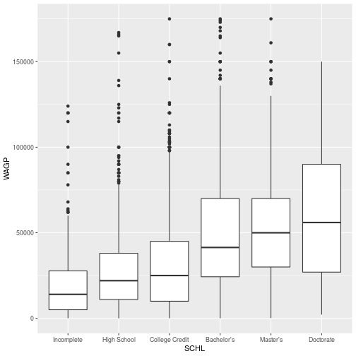
Data visualizations can help confirm intuition, but only with very simple models, typically with just one or two “fixed effects”.
> library(ggplot2)
>
> ggplot(pums,
+   aes(x = SCHL, y = WAGP)) +
+   geom_boxplot()
Within the formula expressions, data transformation functions can also be used.
| Formula | Description |
|---|---|
y ~ log(a) |
log transformed variable |
y ~ sin(a) |
periodic function of a variable |
y ~ I(a*b) |
product of variables, protected by I from expansion |
The WAGP variable is always positive and includes some values that
are many orders of magnitude larger than the mean. Therefore, we can log transform the wages in the model.
fit.schl <- lm(
  log(WAGP) ~ SCHL,
  pums)
> summary(fit.schl)
Call:
lm(formula = log(WAGP) ~ SCHL, data = pums)

Residuals:
    Min      1Q  Median      3Q     Max
-8.3795 -0.4623  0.2330  0.8055  2.5084

Coefficients:
                   Estimate Std. Error t value Pr(>|t|)
(Intercept)         9.21967    0.05861 157.313  < 2e-16 ***
SCHLHigh School     0.54611    0.06816   8.012 1.45e-15 ***
SCHLCollege Credit  0.60397    0.06617   9.127  < 2e-16 ***
SCHLBachelor's      1.22164    0.07243  16.865  < 2e-16 ***
SCHLMaster's        1.36922    0.08615  15.894  < 2e-16 ***
SCHLDoctorate       1.49332    0.22155   6.740 1.79e-11 ***
---
Signif. codes:  0 '***' 0.001 '**' 0.01 '*' 0.05 '.' 0.1 ' ' 1

Residual standard error: 1.19 on 4240 degrees of freedom
Multiple R-squared:  0.09551,	Adjusted R-squared:  0.09444
F-statistic: 89.55 on 5 and 4240 DF,  p-value: < 2.2e-16
Predictor class
For the predictors in a linear model, there is a big difference between factors and numbers.
Compare the model above which fit the wages and level of education (a factor) with one that uses age (a numerical category)
fit.agep <- lm(
  log(WAGP) ~ AGEP,
  pums)
> summary(fit.agep)
Call:
lm(formula = log(WAGP) ~ AGEP, data = pums)

Residuals:
    Min      1Q  Median      3Q     Max
-8.8094 -0.5513  0.2479  0.8093  2.1933

Coefficients:
            Estimate Std. Error t value Pr(>|t|)
(Intercept) 8.842905   0.055483  159.38   <2e-16 ***
AGEP        0.025525   0.001226   20.81   <2e-16 ***
---
Signif. codes:  0 '***' 0.001 '**' 0.01 '*' 0.05 '.' 0.1 ' ' 1

Residual standard error: 1.191 on 4244 degrees of freedom
Multiple R-squared:  0.09261,	Adjusted R-squared:  0.0924
F-statistic: 433.2 on 1 and 4244 DF,  p-value: < 2.2e-16
In the model with AGEP, the intercept and slope is fit. The slope describes the relationship between age and wages and can show a positive, negative, or no relationship between the two variables.
In the model with SCHL, multiple intercepts are fit. The same (Intercept) is fit and 5 intercepts for different factors of SCHL.
As you can see, the SCHL level “Incomplete” is not fit. Each of the SCHL intercepts are based on the “Incomplete” factor, so “Incomplete”” is in theory the (Intercept) coefficient.
For example, the intercept for “SCHLHigh School” is 0.57470, meaning that the log(wages) for someone who completed high school are 0.57 more than someone with incomplete school credit.
Generalized Linear Models
In linear models, like those fit with lm, the distribution of the response variable is assumed to be a normal or gaussian. However, in many cases this assumption is not appropriate.
Generalized linear models allow for other distributions for the response variable, such as binomial or exponential distributions. In generalized linear models, a link function is used to transform the response variable. This causes the response variable to follow a more linear relationship with the predictor variables.
Generalized linear models can be fit in R using the glm function, which is a part of base R. The formula syntax in the lm and glm functions are the same, but an additional argument, family, is used in glm to specify the distribution.
The family argument determines the family of probability distributions in
which the response variable belongs.
| Family | Data Type | (default) link functions |
|---|---|---|
gaussian |
double |
identity, log, inverse |
binomial |
boolean |
logit, probit, cauchit, log, cloglog |
poisson |
integer |
log, identity, sqrt |
Gamma |
double |
inverse, identity, log |
inverse.gaussian |
double |
“1/mu^2”, inverse, identity, log |
The previous model fit with lm is (almost) identical to a model fit using
glm with the Gaussian family and identity link.
fit <- glm(log(WAGP) ~ SCHL,
    family = gaussian,
    data = pums)
> summary(fit)
Call:
glm(formula = log(WAGP) ~ SCHL, family = gaussian, data = pums)

Deviance Residuals:
    Min       1Q   Median       3Q      Max
-8.3795  -0.4623   0.2330   0.8055   2.5084

Coefficients:
                   Estimate Std. Error t value Pr(>|t|)
(Intercept)         9.21967    0.05861 157.313  < 2e-16 ***
SCHLHigh School     0.54611    0.06816   8.012 1.45e-15 ***
SCHLCollege Credit  0.60397    0.06617   9.127  < 2e-16 ***
SCHLBachelor's      1.22164    0.07243  16.865  < 2e-16 ***
SCHLMaster's        1.36922    0.08615  15.894  < 2e-16 ***
SCHLDoctorate       1.49332    0.22155   6.740 1.79e-11 ***
---
Signif. codes:  0 '***' 0.001 '**' 0.01 '*' 0.05 '.' 0.1 ' ' 1

(Dispersion parameter for gaussian family taken to be 1.415141)

    Null deviance: 6633.8  on 4245  degrees of freedom
Residual deviance: 6000.2  on 4240  degrees of freedom
AIC: 13532

Number of Fisher Scoring iterations: 2
- Question
- Should the coefficient estimates between this Gaussian
glm()and the previouslm()be different? - Answer
- It’s possible. The
lm()function uses a different (less general) fitting procedure than theglm()function, which uses IWLS. But with 64 bits used to store very precise numbers, it’s rare to encounter an noticeable difference in the optimum.
Logistic Regression
Calling glm with family = binomial using the default “logit” link performs
logistic regression. We can use this to model the relationship between if an individual has insurance through their employer (HINDS1) and wages (WAGP).
fit <- glm(HINS1 ~ WAGP,
  family = binomial,
  data = pums)
Interpreting the coefficients in the summary of the model is not obvious, but always works
the same way. Looking at the model, you can see that the slope for WAGP is significant.
summary(fit)
Call:
glm(formula = HINS1 ~ WAGP, family = binomial, data = pums)

Deviance Residuals:
    Min       1Q   Median       3Q      Max
-1.1614  -0.8791  -0.6448   1.2314   3.1749

Coefficients:
              Estimate Std. Error z value Pr(>|z|)
(Intercept) -3.765e-02  5.487e-02  -0.686    0.493
WAGP        -2.855e-05  1.692e-06 -16.871   <2e-16 ***
---
Signif. codes:  0 '***' 0.001 '**' 0.01 '*' 0.05 '.' 0.1 ' ' 1

(Dispersion parameter for binomial family taken to be 1)

    Null deviance: 5150.0  on 4245  degrees of freedom
Residual deviance: 4764.9  on 4244  degrees of freedom
AIC: 4768.9

Number of Fisher Scoring iterations: 5
To determine what this means, you have to look at the levels in the HINS1 factor.
levels(pums$HINS1)
[1] "1" "2"
In order, the levels are “1” and “2”, which in the US Census data corresponds to yes and no, respectively for insurance through an employer. For a binomial distribution, the first level of the factor is considered 0 or “failure” and the other levels are considered 1 or “success.” The predicted value, the linear combination of variables and coefficients, is the log odds of “success”. So in this example, HINS1 of 1 (has insurance through employer) is coded as a “0” in the model and HINS1 level of 2 (does not have insurance through employer) is coded as a “1”.
Because the slope of wages in the model is negative, this means that a lower wages corresponds to no insurance through employer.
To make the analysis more intuitive, you can change the order of the levels in the factor so that the level “2” is coded as 0 and the level “1” is coded as 1 or success.
pums$HINS1 <- factor(pums$HINS1, levels = c("2", "1"))
levels(pums$HINS1)
[1] "2" "1"
If you rerun the model, you can see that the estimates remain the same, but the slope of WAGP is not positive, not negative.
fit <- glm(HINS1 ~ WAGP,
  family = binomial,
  data = pums)
> summary(fit)
Call:
glm(formula = HINS1 ~ WAGP, family = binomial, data = pums)

Deviance Residuals:
    Min       1Q   Median       3Q      Max
-3.1749  -1.2314   0.6448   0.8791   1.1614

Coefficients:
             Estimate Std. Error z value Pr(>|z|)
(Intercept) 3.765e-02  5.487e-02   0.686    0.493
WAGP        2.855e-05  1.692e-06  16.871   <2e-16 ***
---
Signif. codes:  0 '***' 0.001 '**' 0.01 '*' 0.05 '.' 0.1 ' ' 1

(Dispersion parameter for binomial family taken to be 1)

    Null deviance: 5150.0  on 4245  degrees of freedom
Residual deviance: 4764.9  on 4244  degrees of freedom
AIC: 4768.9

Number of Fisher Scoring iterations: 5
The always popular \(R^2\) indicator for goodness-of-fit is absent from the
summary of a glm result, as is the default F-Test of the model’s significance.
The developers of glm, detecting an increase in user sophistication, are
leaving more of the model assessment up to you. The “null deviance” and
“residual deviance” provide most of the information we need. To test the fit of a generalized linear model, it is best to compare the deviance of model to the “null model,” which is the model without predictor variables. Therefore, the null model only fits the intercept.
Use a Chi-squared test to see if the deviance in your model is lower than the null model.
anova(fit, update(fit, HINS1 ~ 1), test = 'Chisq')
Analysis of Deviance Table

Model 1: HINS1 ~ WAGP
Model 2: HINS1 ~ 1
  Resid. Df Resid. Dev Df Deviance  Pr(>Chi)
1      4244     4764.9
2      4245     5150.0 -1   -385.1 < 2.2e-16 ***
---
Signif. codes:  0 '***' 0.001 '**' 0.01 '*' 0.05 '.' 0.1 ' ' 1
Linear Mixed Models
The lme4 package expands the formula “mini-language” to allow descriptions of “random effects” into the linear model. These are called mixed models because they contain both fixed and random effects.
- normal predictors are “fixed effects”
(...|...)expressions describe “random effects”
In the context of this package, variables
added to the right of the ~ in the usual way are “fixed effects”—they
consume a well-defined number of degrees of freedom. Variables added within
(...|...) are “random effects”.
Models with random effects should be understood as specifying multiple, overlapping probability statements about the observations.
For example, we can to fit the response variable log(WAGP) with the predictors of marital status (MAR) and education (SCHL), where MAR is a random effect and SCHL is a fixed effect. As assumed by linear models, the response variable, log(WAGP), is normally distributed, with a mean of \mu_i and standard deviation of \sigma_0^2. In addition, the random effect, MAR varies and has a normal distribution, with mean of 0 and standard deviation of \Sigma_1. The fixed effect, SCHL does not vary, and thus is a fixed.
Mixed models can be fit with “random intercepts” and “random slopes”. With a random intercept, each level within the random effect can have a different intercept. With a random slope, each level can have a different slope.
In lme4 random effects are shown in the formula inside parentheses, with variables to the right of a “|” to fit random intercept, and to the left to fit a random slope.
| Formula | Description of random effect |
|---|---|
y ~ (1 | b) + a |
random intercept for each level in b |
y ~ a + (a | b) |
random intercept and slope w.r.t. a for each level in b |
Random Intercept
The lmer function fits linear models with the lme4 extensions to
the lm formula syntax.
library(lme4)
fit <- lmer(
  log(WAGP) ~ (1|MAR) + SCHL,
  data = pums)
> summary(fit)
Linear mixed model fit by REML ['lmerMod']
Formula: log(WAGP) ~ (1 | MAR) + SCHL
   Data: pums

REML criterion at convergence: 12995.7

Scaled residuals:
    Min      1Q  Median      3Q     Max
-7.7980 -0.3802  0.1780  0.6465  2.7135

Random effects:
 Groups   Name        Variance Std.Dev.
 MAR      (Intercept) 0.1491   0.3862
 Residual             1.2398   1.1134
Number of obs: 4246, groups:  MAR, 5

Fixed effects:
                   Estimate Std. Error t value
(Intercept)         9.28460    0.18264  50.835
SCHLHigh School     0.40600    0.06410   6.334
SCHLCollege Credit  0.49035    0.06222   7.881
SCHLBachelor's      0.99794    0.06864  14.539
SCHLMaster's        1.10705    0.08150  13.584
SCHLDoctorate       1.26125    0.20772   6.072

Correlation of Fixed Effects:
            (Intr) SCHLHS SCHLCC SCHLB' SCHLM'
SCHLHghSchl -0.254
SCHLCllgCrd -0.259  0.763
SCHLBchlr's -0.232  0.699  0.719
SCHLMastr's -0.197  0.590  0.607  0.560
SCHLDoctort -0.077  0.231  0.238  0.220  0.186
In a lm or glm fit, each response is conditionally independent, given it’s
predictors and the model coefficients. Each observation corresponds to it’s own
probability statement. Mixed models allow you to specify random effects, assuming that the response variable is not independent given the predictors and model coefficients. In short, mixed models account for the variation due to the random effects and then estimate the coefficients for the fixed effects.
Mixed models are more complicated to interpret. The familiar assessment of model residuals is absent from the summary due to the lack of a widely accepted measure of null and residual deviance. One way to evaluate mixed models is to compare models with different combinations of fixed effects and to the null model.
We can create a null model where we include the random effect of marital status but take out the fixed effect of education.
null.model <- lmer(
  log(WAGP) ~ (1|MAR),
  data = pums)
To compare the fit model to the null model, use the anova function.
anova(null.model, fit)
refitting model(s) with ML (instead of REML)
Data: pums
Models:
null.model: log(WAGP) ~ (1 | MAR)
fit: log(WAGP) ~ (1 | MAR) + SCHL
           npar   AIC   BIC  logLik deviance  Chisq Df Pr(>Chisq)
null.model    3 13310 13329 -6651.8    13304
fit           8 12992 13043 -6488.1    12976 327.37  5  < 2.2e-16 ***
---
Signif. codes:  0 '***' 0.001 '**' 0.01 '*' 0.05 '.' 0.1 ' ' 1
Based on a Chi-squared test, the fit model with education has a lower deviance than the null model, suggesting that education has an effect on wages.
Other factors, such as AIC, BIC, and log likelihood scores are also often used to compare and evaluate mixed models.
Random Slope
Adding a numeric variable on the left of a grouping specified with (...|...)
produces a “random slope” model. Here, separate coefficients for hours worked
are allowed for each level of education.
fit <- lmer(
  log(WAGP) ~ (WKHP | SCHL),
  data = pums)
Warning in checkConv(attr(opt, "derivs"), opt$par, ctrl = control$checkConv, :
unable to evaluate scaled gradient
Warning in checkConv(attr(opt, "derivs"), opt$par, ctrl = control$checkConv, :
Model failed to converge: degenerate Hessian with 1 negative eigenvalues
The warning that the procedure failed to converge is worth paying attention
to. One way to fix this is to change the numerical optimizer used for model fitting
that lme4 is used by default. In this example, we change the optimizer to a “BOBYQA” optimizer, which is slower than the default.
fit <- lmer(
  log(WAGP) ~ (WKHP | SCHL),
  data = pums,
  control = lmerControl(optimizer = "bobyqa"))
> summary(fit)
Linear mixed model fit by REML ['lmerMod']
Formula: log(WAGP) ~ (WKHP | SCHL)
   Data: pums
Control: lmerControl(optimizer = "bobyqa")

REML criterion at convergence: 11658.5

Scaled residuals:
    Min      1Q  Median      3Q     Max
-9.4553 -0.4071  0.1718  0.6258  2.7864

Random effects:
 Groups   Name        Variance  Std.Dev. Corr
 SCHL     (Intercept) 11.856218 3.44329
          WKHP         0.003239 0.05692  -1.00
 Residual              0.900166 0.94877
Number of obs: 4246, groups:  SCHL, 6

Fixed effects:
            Estimate Std. Error t value
(Intercept)  11.2851     0.1084   104.1
The predict function extracts model predictions from a fitted model object
(i.e. the output of lm, glm, lmer, and glmer), providing one easy
way to visualize the effect of estimated coefficients. We can plot the extracted coefficients using ggplot.
ggplot(pums,
  aes(x = WKHP, y = log(WAGP), color = SCHL)) +
  geom_point() +
  geom_line(aes(y = predict(fit))) +
  labs(title = 'Random intercept and slope with lmer')
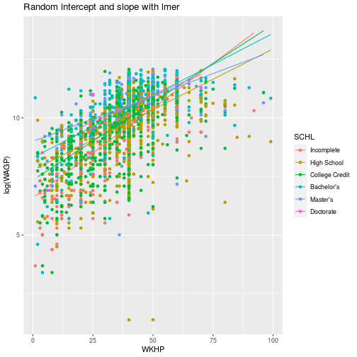
As you can see, each level of education has its own intercept and slope for the best fit line.
Generalized Mixed Models
The glmer function adds upon lmer the option to specify the same group of
exponential family distributions as glm adds to lm. The same family argument is used in glmer to specify the distribution.
A Little Advice
- Don’t start with generalized linear mixed models! Work your way up through
lm()glm()lmer()glmer()
- Take time to understand the
summary()—the hazards of secondary data compel you! The vignettes for lme4 provide excellent documentation.
When stuck, ask for help on Cross Validated. If you are having trouble with lme4, who knows, Ben Bolker himself might provide the answer.
Exercises
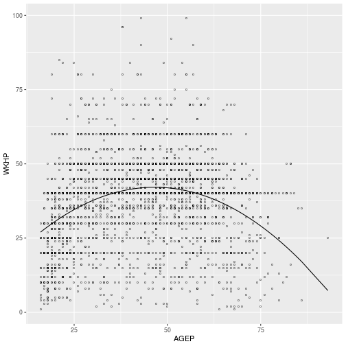
Exercise 1
Regress WKHP against AGEP, adding a second-order interaction to allow for
possible curvature in the relationship. Plot the predicted values over the data
to verify the coefficients indicate a downward quadratic relationship.
Exercise 2
Controlling for a person’s educational attainment, fit a linear model that
addresses the question of wage disparity between men and women in the U.S.
workforce. What other predictor from the pums data frame would increase the
goodness-of-fit of the “control” model, before SEX is considered?
Exercise 3
Set up a generalized mixed effects model on whether a person attained an advanced degree (Master’s or Doctorate). Include sex and age as fixed effects, and include a random intercept according to occupation.
Exercise 4
Write down the formula for a random intercepts model for earned wages with a fixed effect of sex and a random effect of educational attainment.
Solutions
fit <- lm(
  WKHP ~ AGEP + I(AGEP^2),
  pums)

ggplot(pums,
  aes(x = AGEP, y = WKHP)) +
  geom_point(shape = 'o') +
  geom_line(aes(y = predict(fit)))
fit <- lm(WAGP ~ SCHL, pums)
summary(fit)
Call:
lm(formula = WAGP ~ SCHL, data = pums)

Residuals:
   Min     1Q Median     3Q    Max
-61303 -18649  -5649  12990 144351

Coefficients:
                   Estimate Std. Error t value Pr(>|t|)
(Intercept)           19614       1362  14.404  < 2e-16 ***
SCHLHigh School        7396       1584   4.670 3.11e-06 ***
SCHLCollege Credit    11035       1538   7.177 8.34e-13 ***
SCHLBachelor's        29976       1683  17.811  < 2e-16 ***
SCHLMaster's          35197       2002  17.585  < 2e-16 ***
SCHLDoctorate         43889       5148   8.526  < 2e-16 ***
---
Signif. codes:  0 '***' 0.001 '**' 0.01 '*' 0.05 '.' 0.1 ' ' 1

Residual standard error: 27640 on 4240 degrees of freedom
Multiple R-squared:  0.1405,	Adjusted R-squared:  0.1394
F-statistic: 138.6 on 5 and 4240 DF,  p-value: < 2.2e-16
The “baseline” model includes educational attainment, when compared to a model with sex as a second predictor, there is a strong indication of signifigance.
anova(fit, update(fit, WAGP ~ SCHL + SEX))
Analysis of Variance Table

Model 1: WAGP ~ SCHL
Model 2: WAGP ~ SCHL + SEX
  Res.Df        RSS Df  Sum of Sq     F    Pr(>F)
1   4240 3.2391e+12
2   4239 3.0369e+12  1 2.0218e+11 282.2 < 2.2e-16 ***
---
Signif. codes:  0 '***' 0.001 '**' 0.01 '*' 0.05 '.' 0.1 ' ' 1
Adding WKHP to the baseline increases the \(R^2\) to .32 from .14 with just
SCHL. There is no way to include the possibility that hours worked also
dependends on sex, giving a direct and indirect path to the gender wage gap, in
a linear model.
summary(update(fit, WAGP ~ SCHL + WKHP))
Call:
lm(formula = WAGP ~ SCHL + WKHP, data = pums)

Residuals:
   Min     1Q Median     3Q    Max
-82469 -14392  -3970   9369 141498

Coefficients:
                   Estimate Std. Error t value Pr(>|t|)
(Intercept)        -16544.1     1624.9 -10.181  < 2e-16 ***
SCHLHigh School      2874.5     1415.8   2.030   0.0424 *
SCHLCollege Credit   7969.6     1371.2   5.812 6.63e-09 ***
SCHLBachelor's      23859.7     1508.8  15.814  < 2e-16 ***
SCHLMaster's        27986.6     1794.2  15.599  < 2e-16 ***
SCHLDoctorate       34781.5     4588.8   7.580 4.23e-14 ***
WKHP                 1051.9       31.5  33.398  < 2e-16 ***
---
Signif. codes:  0 '***' 0.001 '**' 0.01 '*' 0.05 '.' 0.1 ' ' 1

Residual standard error: 24600 on 4239 degrees of freedom
Multiple R-squared:  0.3195,	Adjusted R-squared:  0.3185
F-statistic: 331.7 on 6 and 4239 DF,  p-value: < 2.2e-16
df <- pums
levels(df$SCHL) <- c(0, 0, 0, 0, 1, 1)
fit <- glmer(
  SCHL ~ (1 | OCCP) + AGEP,
  family = binomial,
  data = df)
anova(fit, update(fit, . ~ . + SEX), test = 'Chisq')
Data: df
Models:
fit: SCHL ~ (1 | OCCP) + AGEP
update(fit, . ~ . + SEX): SCHL ~ (1 | OCCP) + AGEP + SEX
                         npar    AIC    BIC  logLik deviance  Chisq Df
fit                         3 1996.5 2015.6 -995.27   1990.5
update(fit, . ~ . + SEX)    4 1997.6 2023.0 -994.79   1989.6 0.9572  1
                         Pr(>Chisq)
fit
update(fit, . ~ . + SEX)     0.3279
WAGP ~ (1 | SCHL) + SEX
WAGP ~ (1 | SCHL) + SEX
If you need to catch-up before a section of code will work, just squish it's 🍅 to copy code above it into your clipboard. Then paste into your interpreter's console, run, and you'll be ready to start in on that section. Code copied by both 🍅 and 📋 will also appear below, where you can edit first, and then copy, paste, and run again.
# Nothing here yet!