Leaflet in R
Handouts for this lesson need to be saved on your computer. Download and unzip this material into the directory (a.k.a. folder) where you plan to work.
Introduction
Leaflet is a powerful open-source Javascript library that powers interactive maps on the web. This lesson provides an overview of using leaflet, the namesake package in R, to create “slippy” web maps from R and integrate them into RShiny apps.
Like static plotting and mapping, there are lots of options for interactive mapping in R. The leaflet package is actively maintained by RStudio. Some other packages for interactive maps that build off of leaflet, or other interactive plotting libraries, are: tmap, ggiraph, rbokeh, plotly, highcharter, mapedit, mapview, leaflet.extras, and leaflet.esri.
Objectives for this lesson
- Learn how to build leaflet maps with background tiles and layered features
- Customize the appearance of point and shape layers using data attributes
- Get started using leaflet objects in RShiny
What’s a Leaflet?
Leaflet produces maps that have controls to zoom, pan and toggle layers on and off, and can combine local data with base layers from web mapping services.
Maps will appear in RStudio’s Viewer pane, and can also be viewed in a web browser and saved as html files.
The leaflet() function creates an empty leaflet map to which layers can be added using the pipe (%>%) operator. The addTiles() functions adds a base tiled map; by default, it uses tiles made from OpenStreetMap data. Center and set an initial zoom level for the map with setView(). Switch to the “Viewer” tab in RStudio to see the result.
library(leaflet)
leaflet() %>%
addTiles() %>%
setView(lng = -76.505206, lat = 38.9767231, zoom = 7)
Add a new layer with a point marker using addMarkers(), with a custom message that displays when the marker is clicked.
leaflet() %>%
addTiles() %>%
setView(lng = -76.505206, lat = 38.9767231, zoom = 7) %>%
addMarkers(lng = -76.505206, lat = 38.9767231, popup = "I am here!")
In addition to OSM, there are many other data providers that make sets of tiles available to use as basemaps. There is a R list object that loads with leaflet called providers with the names of these options.
leaflet() %>%
addProviderTiles(providers$Esri.WorldImagery) %>%
setView(lng = -76.505206, lat = 38.9767231, zoom = 7) %>%
addMarkers(lng = -76.505206, lat = 38.9767231, popup = "I am here!")
Zoom all the way out. What projection does it look like this map is using?

Read more about the intricacies of web mercator e.g. why it is considered unsuitable for geospatial intelligence purposes. Learn how to define a custom leaflet CRS at RStudio’s guide to working with projections in leaflet.
Layers Control
Layers can be assigned to named groups which can be toggled on and off by the user. baseGroups are selected with radio buttons (where you can only choose one at a time), and overlayGroups get checkboxes.
To implement layers control, add group names to individual layers with the group = argument AND add the layers control layer using addLayersControl().
leaflet() %>%
addTiles(group = "OSM") %>%
addProviderTiles(providers$Esri.WorldImagery, group = "Esri World Imagery") %>%
setView(lng = -76.505206, lat = 38.9767231, zoom = 7) %>%
addMarkers(lng = -76.505206, lat = 38.9767231, popup = "I am here!", group = "SESYNC") %>%
addLayersControl(baseGroups = c("OSM", "Esri World Imagery"),
overlayGroups = c("SESYNC"),
options = layersControlOptions(collapsed = FALSE))
Another type of tile layer is available through many web mapping services (WMS), such as the real-time weather radar data from the Iowa Environmental Mesonet.
leaflet() %>%
addTiles() %>%
setView(lng = -76.505206, lat = 38.9767231, zoom = 5) %>%
addWMSTiles(
"http://mesonet.agron.iastate.edu/cgi-bin/wms/nexrad/n0r.cgi",
layers = "nexrad-n0r-900913",
options = WMSTileOptions(format = "image/png", transparent = TRUE),
attribution = "Weather data © 2012 IEM Nexrad"
)
or USGS topographic maps from the National Map:
nhd_wms_url <- "https://basemap.nationalmap.gov/arcgis/services/USGSTopo/MapServer/WmsServer"
leaflet() %>%
setView(lng = -111.846061, lat = 36.115847, zoom = 12) %>%
addWMSTiles(nhd_wms_url, layers = "0")
Thanks USGS! Check out more USGS Web Mapping Services, and R packages for accessing, processing, and modeling data on github.
In addition to tile layers and markers, many other map features can be added and customized with add*() functions. Refer to the help documentation (eg. ?addMiniMap) to see all of the customization options and learn the default settings.
leaflet() %>%
setView(lng = -111.846061, lat = 36.115847, zoom = 12) %>%
addWMSTiles(nhd_wms_url, layers = "0") %>%
addMiniMap(zoomLevelOffset = -4)
Add layers with common map elements and customize them with add*. Even more new features coming soon!
leaflet() %>%
setView(lng = -111.846061, lat = 36.115847, zoom = 12) %>%
addWMSTiles(nhd_wms_url, layers = "0") %>%
addMiniMap(zoomLevelOffset = -4) %>%
addGraticule() %>%
addTerminator() %>%
addMeasure() %>%
addScaleBar()
Use EasyButtons to add simple buttons that trigger custom JavaScript logic.
The function addEasyButton() adds a simple button to perform an action on your leaflet map.
This map adds one EasyButton to attempt to locate you.
leaflet() %>%
addTiles() %>%
addEasyButton(easyButton(
icon="fa-crosshairs", title = "Locate me",
onClick=JS("function(btn, map){ map.locate({setView: true}); }")))
The onClick argument wraps a little snippet of JavaScript code in the JS function, which
runs when the button is clicked.
The fine print: Note that RStudio’s viewer pane or external window does not always behave the same as a web browser.
Add Data Layers
Spatial objects (points, lines, polygons, rasters) in your R environment can also be added as map layers, provided that they have a CRS defined with a datum. Leaflet will try to make the necessary transformation to display your data in EPSG:3857.
Read in data using sf and raster packages. Points are from the Water Quality Portal accessed via the dataRetrieval package using this script. County boundaries are from the Census and Watershed boundaries are from USGS.
library(sf)
library(raster)
library(dplyr)
wqp_sites <- st_read("data/wqp_sites")
counties_md <- st_read("data/cb_2016_us_county_5m") %>%
filter(STATEFP == "24") %>%
st_transform(4326)
wbd_reg2 <- st_read("data/huc250k/") %>%
filter(REG == "02") %>%
st_transform(4326)
nlcd <- raster("data/nlcd_crop.grd")
Here we use filter to subset the county boundaries to the state with code 24 (Maryland)
and the watershed boundaries to hydrologic unit 02 (Mid-Atlantic). We transform both
to EPSG:4326 (latitude-longitude coordinates with WGS84 datum).
Add a polygons layer, being sure to specify the data = argument. All of the add* layers have “map” as the first argument, facilitating use of the pipe (%>%) operator, but data is not the second argument so it must be named.
leaflet() %>%
addTiles() %>%
addPolygons(data = counties_md)
Customize Polygons with border and fill colors and opacities.
leaflet() %>%
addTiles() %>%
addPolygons(data = counties_md,
color = "green",
fillColor = "gray",
fillOpacity = 0.75,
weight = 1)
Attributes can be referred to using formula syntax ~ to access attribute data from an sf object or Spatial*DataFrame. What is the difference between a popup and a label?
leaflet() %>%
addTiles() %>%
addPolygons(data = counties_md, popup = ~NAME, group = "click") %>%
addPolygons(data = counties_md, label = ~NAME, group = "hover") %>%
addLayersControl(baseGroups = c("click", "hover"))
Notice that the names "click" and "hover" that we assigned to the groups correspond to the different behavior of popups and labels!
For numeric or categorical data, create a color palette from colorbrewer using colorNumeric(), colorFactor(), colorBin(), or colorQuantile().
pal <- colorNumeric("PiYG", wbd_reg2$AREA)
leaflet() %>%
addTiles() %>%
addPolygons(data = wbd_reg2,
fillColor = ~pal(AREA),
fillOpacity = 1,
weight = 1)
Load the RColorBrewer library to see information about palettes in the brewer.pal.info data.frame.
Leaflet’s color palette syntax can be a little confusing. The functions called color*() return another function, so here the object pal is a custom-defined function that maps a numeric value to a color. In this case the range of values in wbd_reg2$AREA is mapped to the range of colors in the "PiYG" palette. Then we use formula notation, ~pal(AREA), to tell addPolygons() that the fillColor should be computed for each polygon by applying the function pal() to the AREA value of that polygon.
Add a legend (which will likely duplicate arguments from the layer that used that palette).
leaflet() %>%
addTiles() %>%
addPolygons(data = wbd_reg2,
fillColor = ~pal(AREA),
fillOpacity = 0.9,
weight = 1) %>%
addLegend(pal = pal, values = wbd_reg2$AREA, title = "Watershed Area")
Add points as markers, circle markers, or customized icons.
leaflet() %>%
addTiles() %>%
addMarkers(data = wqp_sites[1:1000,], group = "markers") %>%
addCircleMarkers(data = wqp_sites[1:1000,], radius = 5, group = "circlemarkers") %>%
addLayersControl(baseGroups = c("markers", "circlemarkers"))
Here the radius argument indicates the size of the "circlemarkers" group.
Display a different number of markers at each zoom level using clusterOptions on markers or circle markers layers.
leaflet() %>%
addTiles() %>%
addMarkers(data = wqp_sites, clusterOptions = markerClusterOptions(),
popup = ~paste(MntrnLN, ",", OrgnztI))
Here, we use the function markerClusterOptions() with all default arguments. This will use pre-defined logic to decide
how many markers to collapse together at each zoom level. The popup argument will only
show the popup text when you are zoomed in far enough to click on an individual marker.
Rasters can be slow to load. Be patient but also check out the maxBytes = argument if need be.
leaflet() %>%
addTiles() %>%
addRasterImage(nlcd)
Warning in raster::projectRaster(x, raster::projectExtent(x, crs =
sp::CRS(epsg3857)), : input and ouput crs are the same
Publish a Leaflet Map
You can render a map and publish it as an HTML file using the htmlwidgets package.
Your HTML map can be used as a standalone website or embedded in an existing website.
Create a map centered on Annapolis and add a weather data tile.
library(htmlwidgets)
map <- leaflet() %>%
addTiles() %>%
setView(lng = -76.505206, lat = 38.9767231, zoom = 5) %>%
addWMSTiles(
"http://mesonet.agron.iastate.edu/cgi-bin/wms/nexrad/n0r.cgi",
layers = "nexrad-n0r-900913",
options = WMSTileOptions(format = "image/png", transparent = TRUE),
attribution = "Weather data © 2012 IEM Nexrad"
)
Now that we have a map, let’s save it by using the saveWidget()function.
saveWidget() will save your map to your working directory as a .html file.
saveWidget(map, file="map.html")
You can now open map.html in your browser as a full-screen html file.
To share your map, you can upload the html file to GitHub or any web server.
We suggest you use GitHub Pages to share your map.
To publish your map on GitHub Pages, do the following:
- Create a repository on GitHub.
- Rename your
map.htmlfile toindex.htmland push this file to your repository. - Go to your repository’s settings and enable GitHub Pages.
- After a few minutes, your page will be ready to go and a link will be provided.
Your map is now live. You can now share the link with your colleagues to share your map!
For more information about GitHub Pages, including a walkthrough of the steps above, please see our lesson on Advanced git Techniques. For information on getting started with GitHub, check out our Basic git lesson.
If you prefer to embed your map inside a project, personal, or any other website you can do so by using the html <iframe> tag.
<iframe src="map.html" frameborder="0" width="50%" height="200px"></iframe>
This is a good option when you already have a site built and would like to add your map to share it.
Web development is out of the scope of this lesson, but please check this tutorial out if you would like to learn more about using the iframe tag in your websites.
Leaflet in Shiny
Shiny is a web application framework for R that allows you to create interactive web apps without requiring knowledge of HTML, CSS, or JavaScript.
These web apps can be used for exploratory data analysis and visualization, to facilitate remote collaboration, share maps, and much more.
Incorporating leaflet maps into Shiny applications allows for creating more customized interactivity using R code.
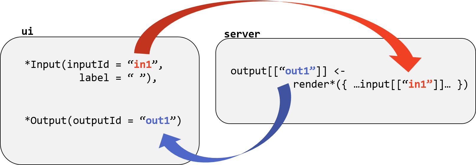
As you may have learned in the Shiny lesson, the app comprises a user interface object that defines how it appears, and a server object that defines how it behaves.
The ui and server interact through *input and *output objects such as input widgets, plots, buttons, tables, etc.
The example below represents a basic Shiny app.
library(shiny)
# Define the user interface
ui <- navbarPage(title = 'Hello, Shiny World!')
# define the server component
server <- function(input, output){}
# Create the app
shinyApp(ui = ui, server = server)
We start by defining the ui. In this case, we use the navbarPage() function to define a navigation bar object to display the “Hello, Shiny World!” text.
Next we define the server component, a custom function that specifies the behavior of the app. The server function takes in two parameters, an input and an output. In the example above, the server function is currently empty, so our app doesn’t do anything, but we will cover this shortly.
Leaflet maps in Shiny are constructed with renderLeaflet() and displayed in the output using leafletOutput().
To see how all of this works, we’ll build a shiny app with a leaflet map, where one of the map layers is defined with a user-specified value from an input widget. See the app in action here.
Define an output object called map in the server function.
server <- function(input, output) {
# renderLeaflet created the map widget for the app
output$map <- renderLeaflet({
# leaflet map is defined here with tiles, initial view, and layer control options
leaflet() %>%
addTiles(group = "OSM") %>%
addProviderTiles(providers$NASAGIBS.ModisTerraTrueColorCR, group = "Modis",
options = providerTileOptions(time = "2018-01-05")) %>%
setView(lng = -76.505206, lat = 38.9767231, zoom = 7) %>%
addLayersControl(baseGroups = c("Modis", "OSM"),
options = layersControlOptions(collapsed = FALSE)
)
})
}
We wrap the leaflet map inside the renderLeaflet() function, using curly brackets {} around the expression.
We include two tile layers, OpenStreetMap and MODIS imagery, with addLayersControl activated to
allow the user to select which one to display.
output$map is assigned the map widget for the app rendered by the renderLeaflet function.
Define the ui to include the output called "map".
ui <- fluidPage(
leafletOutput("map", height = 800)
)
Remember, the ui is the page that humans interact with. In this case, it is a fluid page containing the map. We include the output of the leafletOutput() function, the map rendered in the server function, and add it to the apps page.
A fluidPage() is a browser window where the contents scale up or down as the window size is changed.
Add a panel to the ui that will let users choose a calendar date.
ui <- fluidPage(
leafletOutput("map", height = 800),
# add calendar panel
absolutePanel(top = 100, right = 10, draggable = TRUE,
dateInput("dateinput", "Imagery Date", value = "2018-03-28"
)
))
We have the map and now we add a calendar panel to let the user pick a date. We use dateInput() to define the panel type and set the panel position with the absolutePanel() function. You’ll notice that we have defined the an input id, a label, and a initial value for the panel widget inside the dateInput() function. The input id will be used to access the value, date, set by the user in the server function. The
next argument, label, is the descriptive title seen by the user, and the value
argument is the starting value before user input.
Use the dateinput input object in the Provider Tiles layer.
addProviderTiles(providers$NASAGIBS.ModisTerraTrueColorCR, group = "Modis",
options = providerTileOptions(time = input$dateinput))
Now, the MODIS tiles will be retrieved for a user-input day specified by
providerTileOptions(). The MODIS tile provider accepts an option called
time to which we pass the dateinput object from the list called input
that the server function gets from the ui.
Display your app.
shinyApp(ui, server)
A new window with your leaflet map app will be launched. The shinyApp() function creates a Shiny app from an ui/server pair.
Refer to our Shiny Apps lesson to learn more about Shiny.
We now are able to publish your map via a Shiny app! However, the app is hosted locally and can only be viewed on your local machine.
To share your map and Shiny app with others, first make sure everything the app needs to run (data and packages) is loaded into the R session.
You can share your Shiny app as files. This is limited and requires users to have R installed on their computers.
- Directly share the source code (app.R, or ui.R and server.R) along with all required data files.
- Your app user can place the files into a local directory.
- They can launch the app in R by running
runApp("appFolderName")library(shiny) runApp("coolApp")
- Publish the files to a GitHub repository, and advertise that your app can be cloned and run with
runGitHub('<USERNAME>/<REPO>')- Create a directory for your app
- Share directory with app users and instruct to clone it
- Run app with
runGitHub()library(shiny) runGitHub("<USERNAME>/<REPO>")
You can share your Shiny app as a web page. This is the preferred way to share Shiny apps since users do not need to have R installed on their computers.
To share just the UI (i.e. the web page), your app will need to be hosted by a server able to run the R code that powers the app while also acting as a public web server. There is limited free hosting available through RStudio with shinyapps.io.
Check out these series of articles on the RStudio website about deploying apps or this tutorial on sharing Shiny apps.
Shiny Optimization
Rendering maps can be slow.
Use leafletProxy() so the whole map doesn’t have to be re-drawn every time the user input is updated.
leafletProxy() allows for finer-grained control over a map, such as changing the color of a single polygon or adding a marker at the point of a click – without redrawing the entire map.
It is good practice to modify a map that’s already running in a Shiny app with a leafletProxy() function call in place of the leaflet() call, but otherwise use Leaflet function calls as normal.
Let’s make a new shiny app that only changes one map layer when a new value is selected from an input widget.
See the app in action here.
Read in data for watershed boundaries for the mid-Atlantic region of the USA.
wbd_reg2 <- st_read("https://raw.githubusercontent.com/khondula/leaflet-in-R-shinydemo2/master/data/wbd_reg2.geojson") %>%
filter(REG == "02") %>%
st_transform(4326)
We filter the GeoJSON shapefile to a single region polygon (code "02" is the mid-Atlantic) and transform to EPSG:4326 latitude-longitude coordinate system.
Define the user interface of the Shiny app. A map and an input panel to select a color scheme for the layer is defined.
# user interface with map and color scheme widget
ui <- fluidPage(
leafletOutput("map", height = 800),
absolutePanel(top = 10, right = 10, draggable = TRUE,
selectInput(inputId = "colors",
label = "Color Scheme",
choices = row.names(brewer.pal.info))
))
Define the server.
# server definition
server <- function(input, output) {
output$map <- renderLeaflet({
# use this line with leafletproxy for default colors
pal <- colorNumeric("BrBG", wbd_reg2$AREA)
# map with polygons and legend
leaflet() %>%
addTiles() %>%
setView(lng = -76.505206, lat = 38.9767231, zoom = 7) %>%
addPolygons(data = wbd_reg2,
fill = TRUE,
color = "black",
weight =1,
fillColor = ~pal(AREA), # color is function of the wbd AREA column
fillOpacity = 0.8,
popup = ~HUC_NAME) %>%
addLegend(position = "bottomright", pal = pal, values = wbd_reg2$AREA)
})
# update map using leaflet proxy instead of recreating the whole thing
# use observe to color layer as needed
observe({
# color palette is defined according to the user's input
pal <- colorNumeric(input$colors, wbd_reg2$AREA)
# the map is updated with the new prefered color palette
# notice we use leafletProxy() instead of leaflet()
leafletProxy("map") %>%
clearShapes() %>% clearControls() %>%
addPolygons(data = wbd_reg2, fill = TRUE,
color = "black", weight =1,
fillColor = ~pal(AREA),
fillOpacity = 0.8,
popup = ~HUC_NAME) %>%
addLegend(position = "bottomright", pal = pal, values = wbd_reg2$AREA)
})
}
Incremental changes to the map (in this case, replacing the color of the watershed boundaries) should be performed in an observer. Each independent set of things that can change should be managed in its own observer.
Run the app using shinyApp(ui, server) and zoom in or out. What happens when you change the color scheme?
In summary, use leafletProxy to change, customize, and control, a map that has already been rendered.
Normally, you create a Leaflet map using the leaflet() function. This creates an in-memory representation of a map that you can customize using functions like addPolygons() and setView(). Such a map can be printed at the R console, included in an R Markdown document, or rendered as a Shiny app.
In the case of Shiny, you may want to further customize a map, even after it is rendered to an output. At this point, the in-memory representation of the map is long gone, and the user’s web browser has already realized the Leaflet map instance.
This is where leafletProxy() comes in. It returns an object that can stand in for the usual Leaflet map object. The usual map functions like addPolygons and setView can be called, and instead of customizing an in-memory representation, these commands will execute on the live Leaflet map instance, optimizing your map!
Summary
We have covered:
- how to build an interactive map using
Leaflet - how to publish a Leaflet map using HTML and Github
- how to integrate and publish a Leaflet map with
Shiny
Main functions for leaflet maps
- View window -
setView(lat, lon, zoom)fitBounds()setMaxBounds() - Background tiles -
addTiles()addProviderTiles()addWMSTiles() - Point layers -
addMarkers()addCircleMarkers()addAwesomeMarkers()addLabelOnlyMarkers() - Shape layers -
addPolylines()addCircles()addRectangles()addPolygons() - Images -
addRasterImage() - Common features -
addLegend()addLayersControl()addControl()
For HTML
saveWidget(map, file="map.html")saves your map object as an html file which can be loaded in a browser.- Use
iframeto embed the map html file to your website and share it :).
For Shiny apps
renderLeaflet()objects in the server and use them in the ui withleafletOutput()- Use
shinyApp()to display your map with Shiny. - Host your app on GitHub or another web server and share your app.
- Optimize your Shiny maps using
leafletProxy()
Exercises
Exercise 1
Create a leaflet map with a marker at a location and zoom level of your choice that includes
- Background imagery from a tile provider of your choice (Hint: browse options in the
providerslist) - A label that appears when the mouse hovers over the marker (Hint: use the
labelargument toaddMarkers())
Exercise 2
Create a leaflet map with default background imagery and the counties_md polygons colored by land area (the ALAND column),
using the "Oranges" palette. Set fillOpacity = 1 to make the colors more visible.
Hint: You will need to define a palette function using colorNumeric() before you create the map.
The first argument to colorNumeric() should be the name of the palette ("Oranges"),
and the second argument is the range of values to map to colors (counties_md$ALAND).
Exercise 3
Modify the Shiny app on worksheet 3 (the app where the user selects a date of MODIS imagery to display) to do the following:
- Always display both the OpenStreetMap and MODIS layers, instead of letting the user choose.
- Include a slider labeled “Set Opacity” that will allow the user to modify the variable
input$opacity. - Use the variable
input$opacityto set the opacity of the MODIS layer between 0 and 1, with the default value being 1.
This is challenging so don’t be afraid to look at the hints!
Hints:
- Remove the
addLayersControl()function entirely to disable the switching on and off of layers. - Add another argument to
absolutePanel()after thedateInput(). This argument will besliderInput(). - The arguments to
sliderInput()should be the input variable name ("opacity"), the label that the user will see ("Set Opacity"), the minimum value (min = 0), the maximum value (max = 1), and the default value (value = 1). - Finally, add another argument to
providerTileOptions()to set the opacity (opacity = input$opacity).
Solutions
Solution 1
This is an example solution centered on the Washington Monument, zoomed in to level 14, with Stamen.Toner background imagery.
> lng <- -77.0351929
> lat <- 38.8894791
> leaflet() %>%
+ setView(lng = lng, lat = lat, zoom = 14) %>%
+ addProviderTiles(providers$Stamen.Toner) %>%
+ addMarkers(lng = lng, lat = lat, label = "Yep, that's it")
Solution 2
> pal <- colorNumeric('Oranges', counties_md$ALAND)
> leaflet() %>%
+ addTiles() %>%
+ addPolygons(data = counties_md,
+ fillColor = ~ pal(ALAND),
+ fillOpacity = 1)
Solution 3
Notice that on line 6 of this script, the sliderInput() is added as an extra argument after the dateInput(), so the slider appears just
below the date selector in the input panel.
Also notice that on line 16, providerTileOptions() has two arguments, time and opacity, both of which get values
from the input variable that the user can modify.
> ui <- fluidPage(
+ leafletOutput("map", height = 800),
+ # add calendar panel
+ absolutePanel(top = 100, right = 10, draggable = TRUE,
+ dateInput("dateinput", "Imagery Date", value = "2018-03-28"),
+ sliderInput("opacity", "Set Opacity", min = 0, max = 1, value = 1)
+ ))
>
> server <- function(input, output) {
+
+ output$map <- renderLeaflet({
+ # leaflet map is defined here with tiles and initial view, and no layer control
+ leaflet() %>%
+ addTiles(group = "OSM") %>%
+ addProviderTiles(providers$NASAGIBS.ModisTerraTrueColorCR, group = "Modis",
+ options = providerTileOptions(time = input$dateinput, opacity = input$opacity)) %>%
+ setView(lng = -76.505206, lat = 38.9767231, zoom = 7)
+ })
+
+ }
>
> shinyApp(ui, server)
If you need to catch-up before a section of code will work, just squish it's 🍅 to copy code above it into your clipboard. Then paste into your interpreter's console, run, and you'll be ready to start in on that section. Code copied by both 🍅 and 📋 will also appear below, where you can edit first, and then copy, paste, and run again.
# Nothing here yet!