Advanced Tidyverse
Note: This lesson is in beta status! It may have issues that have not been addressed.
Handouts for this lesson need to be saved on your computer. Download and unzip this material into the directory (a.k.a. folder) where you plan to work.
Lesson Objectives
- Meet the core tidyverse
- Learn functions that ease data cleaning
- Level up in exploratory data viz
Specific Achievements
- Read a folder of tabular files into one data frame
- Efficiently manipulate string and date vectors
- Format ggplot labels with markdown syntax
- Rearrange and find all combinations of factor levels
Review and Pre-Requisites
You should have already be familiar with these topics:
What is the tidyverse?
The tidyverse is an opinionated collection of R packages designed for data science. There are multiple packages designed to tackle each stage of the data science workflow (depicted below), unified by common design philosophies and data structures.
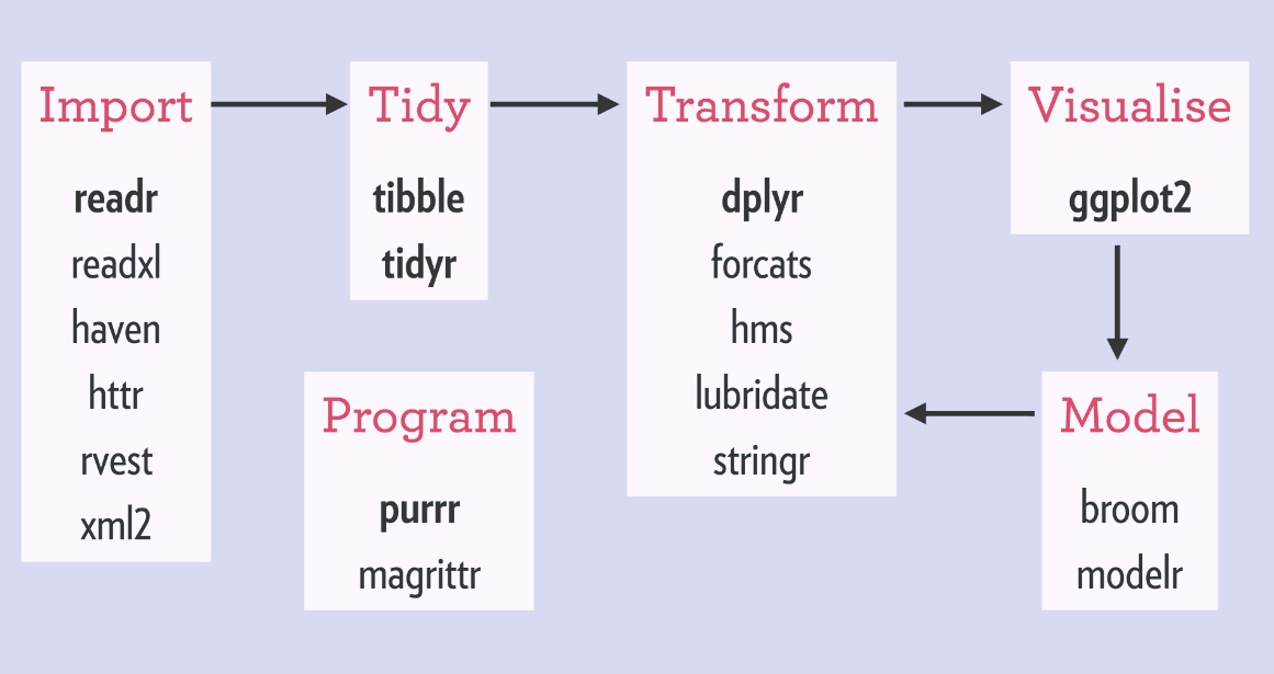
How tidyverse packages fit into a canonical data science workflow. source
Because packages share a high-level design philosophy and low-level grammar and data structures, learning one package should make it easier to learn the next. Tidyverse packages are designed to work best with tidy data frames, and emphasize readability, consistency, and modularity.
These are not strictly alternatives but you might compare it to using either: only using base R, which prioritizes stability (i.e. doesn’t change as quickly), or data.table, which prioritizes speed and concise syntax.
If you want to up with new developments in the tidyverse, check out the blog, videos from the RStudio conferences, or follow the developers on Twitter.
Core Tidyverse
Load the tidyverse meta-package using:
library(tidyverse)
── Attaching packages ─────────────────────────────────────── tidyverse 1.3.1 ──
✓ ggplot2 3.3.5     ✓ purrr   0.3.4
✓ tibble  3.1.6     ✓ dplyr   1.0.7
✓ tidyr   1.1.3     ✓ forcats 0.5.1
✓ readr   2.0.1
── Conflicts ────────────────────────────────────────── tidyverse_conflicts() ──
x dplyr::filter() masks stats::filter()
x dplyr::lag()    masks stats::lag()
This loads the 8 “core” tidyverse packages into your environment:
| Package | Purpose | Prominent functions |
|---|---|---|
readr |
read flat files | read_csv, write_csv |
tidyr |
reshaping | pivot_longer, pivot_wider |
dplyr |
wrangling | filter, select, summarize |
ggplot2 |
visualization | ggplot, aes |
stringr |
control character vectors | str_sub, str_pad |
tibble |
opinionated data frames | glimpse, rownames_to_column |
forcats |
categorical data | fct_relevel, fct_anon |
purrr |
iteration | map, walk, pmap |
Expanded tidyverse
When you run install.packages("tidyverse") it also installs a number of other packages with more specialized uses, as well as many package dependencies such as fs and scales.
| Purpose | Packages |
|---|---|
| Importing data | DBI, dbplyr, haven, httr, readxl, rvest, jsonlite, xml2 |
| Wrangling specific types of data | lubridate, hms, blob |
| General programming | magrittr, glue, reprex, rlang |
| Modeling | broom, modelr |
| Under the hood | pillar, rlang, cli, crayon |
Use tidyverse_deps(recursive = TRUE) to see a list of all 89 tidyverse packages and dependencies.
Loading data
This lesson uses data modified from the palmerpenguins package, which provides a dataset about 3 penguin species collected at Palmer Station Antarctica LTER.
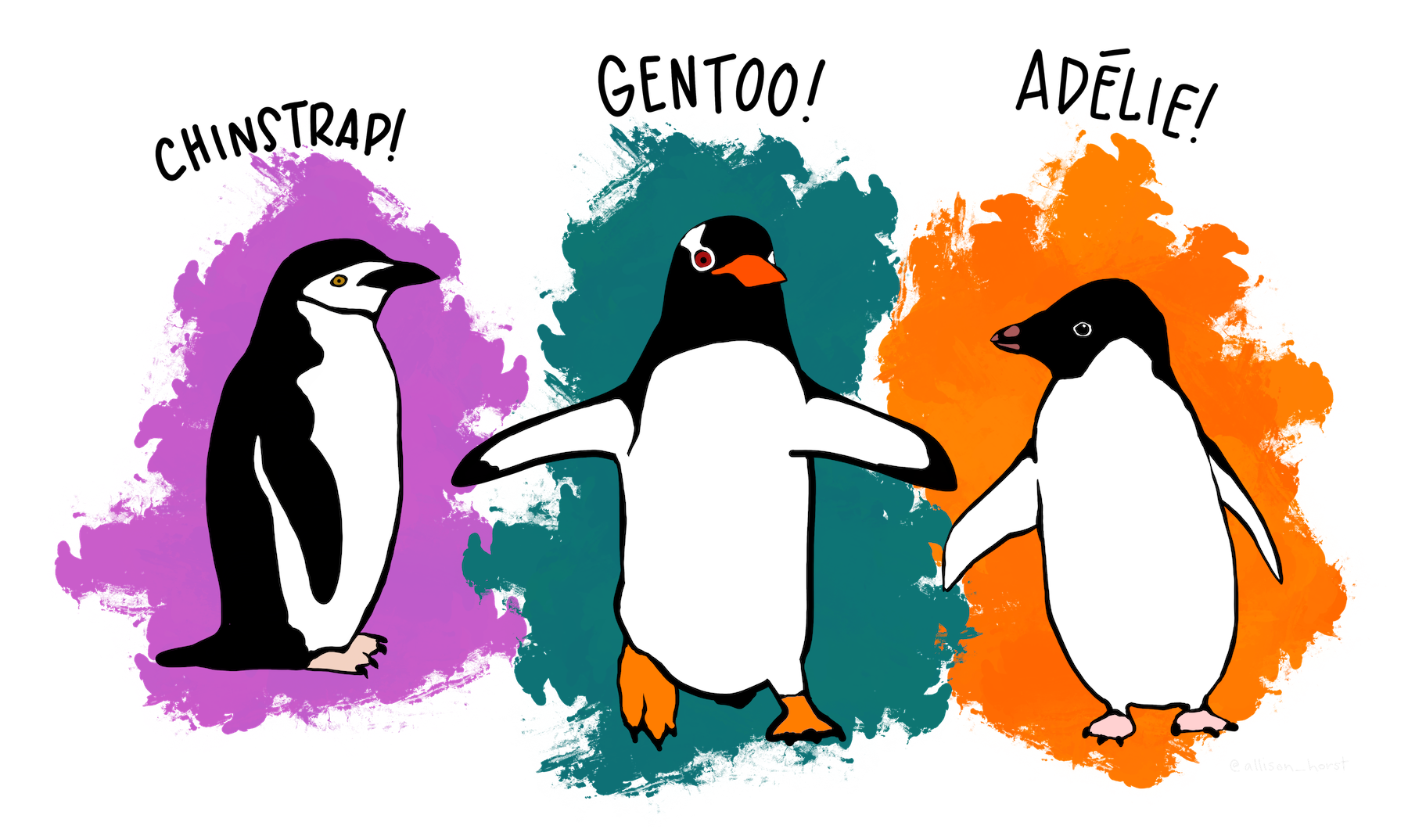
Credit: Artwork by @allison_horst
For this lesson, the data has been split up into separate files – one for each study date when nests were observed. The sampling date is included in the file name but not in the data itself. Each row contains data on characteristics and measurements associated with one observation of a study nest.
Our goal is to read in all 50 of those files from the penguins folder into one data frame, and add the sampling date from each file name in the data. We will do this using map functions in purrr, the tidyverse workhorse for iteration. The inputs we will need are:
- (1) a list of objects to iterate over, and
- (2) the function to apply to each one.
Before seeing purrr::map in action, we will explore the inputs.
The list of objects to iterate over is a vector of file names, which can be created using dir_ls in fs. This package contains functions to work with files, filepaths, and directories. Most functions are named based on their unix equivalent, with the corresponding prefix file_, path_, or dir_.
Create a vector with all of the file names in the data/penguins folder:
library(fs)
penguin_files <- dir_ls('data/penguins')
If we were interested in only a subset of files in that directory, we could filter them by supplying a pattern to the argument glob or regexp, such as “only files with the word penguin in the name ending in .csv”.
> dir_ls('data/penguins', glob = "*penguins*.csv")
The function to apply to each of the file names is read_csv in readr, such as
> read_csv(file = penguin_files[1])
Rows: 8 Columns: 17
── Column specification ────────────────────────────────────────────────────────
Delimiter: ","
chr (10): studyName, Region, Island, Stage, Individual ID, Clutch Completion...
dbl  (7): Sample Number, Culmen Length (mm), Culmen Depth (mm), Flipper Leng...
ℹ Use `spec()` to retrieve the full column specification for this data.
ℹ Specify the column types or set `show_col_types = FALSE` to quiet this message.
# A tibble: 8 × 17
  studyName `Sample Number` Region Island Stage `Individual ID` `Clutch Complet…
  <chr>               <dbl> <chr>  <chr>  <chr> <chr>           <chr>
1 PAL0910                93 Anvers Biscoe Adul… N18A1           Yes
2 PAL0910                94 Anvers Biscoe Adul… N18A2           Yes
3 PAL0910               105 Anvers Biscoe Adul… N24A1           Yes
4 PAL0910               106 Anvers Biscoe Adul… N24A2           Yes
5 PAL0910               117 Anvers Biscoe Adul… N36A1           Yes
6 PAL0910               118 Anvers Biscoe Adul… N36A2           Yes
7 PAL0910               119 Anvers Biscoe Adul… N38A1           No
8 PAL0910               120 Anvers Biscoe Adul… N38A2           No
# … with 10 more variables: Culmen Length (mm) <dbl>, Culmen Depth (mm) <dbl>,
#   Flipper Length (mm) <dbl>, Body Mass (g) <dbl>, Sex <chr>,
#   Delta 15 N (o/oo) <dbl>, Delta 13 C (o/oo) <dbl>, Comments <chr>,
#   common <chr>, latin <chr>
Note in the output message that the object created is a tibble, which is slightly different than a typical data frame. For example, the displayed portion in the console is easier to read and contains the data type in each column.
As also suggested by the output message, the data type for each column is determined automatically. The default parses the first 1,000 rows of the table, but the col_types argument offers more control. One way to specify column types is a character string the same length as the number of columns:
| character | data type |
|---|---|
c |
character/string |
i |
integer |
n |
numeric |
d |
double |
l |
logical |
f |
factor/categorical |
D |
date |
T |
date time |
t |
time |
? |
guess |
_ or - |
skip this column |
pg_df1 <- read_csv(penguin_files[1], col_types = "cdcccccddddcddccc")
Or use spec_csv to generate a column specification object that can be passed to the col_types argument.
my_col_types <- spec_csv(penguin_files[1])
> my_col_types
cols(
  studyName = col_character(),
  `Sample Number` = col_double(),
  Region = col_character(),
  Island = col_character(),
  Stage = col_character(),
  `Individual ID` = col_character(),
  `Clutch Completion` = col_character(),
  `Culmen Length (mm)` = col_double(),
  `Culmen Depth (mm)` = col_double(),
  `Flipper Length (mm)` = col_double(),
  `Body Mass (g)` = col_double(),
  Sex = col_character(),
  `Delta 15 N (o/oo)` = col_double(),
  `Delta 13 C (o/oo)` = col_double(),
  Comments = col_character(),
  common = col_character(),
  latin = col_character()
)
Map functions
The approach to iteration in the tidyverse is map functions in purrr. Compared to *apply functions, these offer predictable return objects and consistent syntax.
The arguments to map are:
.x- a list of things to iterate over.f- what to do for each item in.x
.f can be either the name of an existing function, or an “anonymous” function created from a formula.
Read each of the penguin_files into a list using ~ formula syntax:
pg_list <- map(.x = penguin_files, .f = ~ read_csv(.x, col_types = my_col_types))
Whereas map always returns a list, map_* functions return specific types of vectors such as map_chr for character vectors or map_intfor integer vectors. Use map_dfr for returning one dataframe:
pg_df <- map_dfr(penguin_files, ~read_csv(.x, col_types = my_col_types))
Another handy argument for map_dfr is .id, which adds a column with the names of each item in .x.
pg_df <- map_dfr(penguin_files, ~read_csv(.x), .id = "filename")
Combine operations with pipes
Remember the %>% ?
Readability is one of the core tenets of the tidyverse and this is accomplished with piped workflows. The functions are designed to work together based on the first argument and the type of output returned.
Let’s combine our previous steps together without creating intermediate objects:
pg_df <- dir_ls("data/penguins") %>%
  map_dfr(~read_csv(.x), .id = "filename")
This code creates a vector of file names with dir_ls(), and then “maps” the read_csv() function over each file. The output of each read_csv() function is row-binded (i.e. combined) together into one dataframe called pg_df, with an additional column containing the filename that each row of data came from.
Manipulate strings and dates
Another core tenet of the tidyverse is tidy evaluation, which facilitates:
- using names of data variables as if they were variables in your environment (referred to as data masking)
- identifying variables based on their position, name, or type (referred to as tidy selection)
In base R there is similar functionality using attach(pg_df) or data = pg_df arguments in functions like lm. Tidyverse functions take those ideas and make them consistent and operational in a reliable manner beyond usage in interactive programming.
Given this focus on variable names, let’s make it easier to use them without special syntax by renaming the columns of pg_df to remove spaces and punctuation.
> names(pg_df)
 [1] "filename"            "studyName"           "Sample Number"
 [4] "Region"              "Island"              "Stage"
 [7] "Individual ID"       "Clutch Completion"   "Culmen Length (mm)"
[10] "Culmen Depth (mm)"   "Flipper Length (mm)" "Body Mass (g)"
[13] "Sex"                 "Delta 15 N (o/oo)"   "Delta 13 C (o/oo)"
[16] "Comments"            "common"              "latin"
Within dplyr functions like rename where the data frame is always the first argument, tidy eval means you don’t need to re-specify the data frame name when you refer to a specific column. For example, rename the column “studyName” to “study_name”
pg_df <- rename(pg_df, study_name = studyName)
Instead of changing each column individually, rename_with is a handy shortcut to do the same modification to all (or a collection of) column names. The arguments are:
- a data frame
- a function to apply to each column name
- a selection of column to rename (by default all columns)
Manipulating strings
Before changing the names, we will test out functions in stringr for manipulating character strings. Common tasks often involve pattern matching, which can be accomplished by specifying either an exact match, or via regular expressions.
For example, replace all of the spaces in a character string using either:
str_replace_all("Body Mass (g)", pattern = " ", replacement = "_")
[1] "Body_Mass_(g)"
str_replace_all("Body Mass (g)", pattern = "[:space:]", replacement = "_")
[1] "Body_Mass_(g)"
The regex pattern [:punct:] is a concise way to match all punctuation symbols at once.
str_replace_all("Delta 15 N (o/oo)", pattern = "[:punct:]", replacement = "")
[1] "Delta 15 N ooo"
Use these functions as arguments to a piped sequence of rename_with functions to combine both transformations and convert to lower case in one fell swoop:
pg_df <- pg_df %>%
  rename_with(~str_replace_all(.x, "[:punct:]", "")) %>%
  rename_with(~str_replace_all(.x, "[:space:]", "_")) %>%
  rename_with(~str_to_lower(.x))
> names(pg_df)
 [1] "filename"          "studyname"         "sample_number"
 [4] "region"            "island"            "stage"
 [7] "individual_id"     "clutch_completion" "culmen_length_mm"
[10] "culmen_depth_mm"   "flipper_length_mm" "body_mass_g"
[13] "sex"               "delta_15_n_ooo"    "delta_13_c_ooo"
[16] "comments"          "common"            "latin"
Much improved!! Note that a more robust method of creating syntactic names can be accomplished using the .name_repair argument in tibble::tibble or readxl::read_excel.
Format dates
Now let’s work on putting the date information from the filenames into a properly formatted column of dates. Look at a sample of the data to evaluate: Is there a systematic way to extract the necessary information?
> sample(pg_df$filename, 5)
[1] "data/penguins/penguins_nesting-December-3-2007.csv"
[2] "data/penguins/penguins_nesting-November-16-2009.csv"
[3] "data/penguins/penguins_nesting-December-3-2007.csv"
[4] "data/penguins/penguins_nesting-November-28-2007.csv"
[5] "data/penguins/penguins_nesting-November-15-2009.csv"
We can use pattern matching to identify and remove “data/penguins/penguins_nesting-“ or (|) “.csv” using str_remove_all. Save a new vector to use for testing out date conversions.
egg_dates <- str_remove_all(string = pg_df$filename,
    pattern = "(data/penguins/penguins_nesting-)|(.csv)")
lubridate facilitates working with date formats. Can as_date automatically interpret “December-1-2009” as a date?
library(lubridate)
Attaching package: 'lubridate'
The following objects are masked from 'package:base':

    date, intersect, setdiff, union
egg_dates[1] %>% as_date()
Warning: All formats failed to parse. No formats found.
[1] NA
As with the base as.Date function, unless dates are already specified using the ISO 8601 YYYY-MM-DD representation, date conversion with lubridate::as_date requires a character string defining the date using codes from the POSIX standard:
| code | meaning |
|---|---|
%b |
Abbreviated month name in current locale |
%B |
Full month name in current locale |
%d |
Day of month as decimal number (01-31) |
%j |
Day of year as decimal number (001-366) |
%y |
Year without century (00-99) |
%Y |
Year with century |
Note that interpretation of many POSIX codes depend on settings of your operating system, such as month or weekday names in different languages, whether weeks start on Sunday or Monday, or the default century for %y. Read more about format specification in the Details section of the base strptime function.
> ?strptime
Supply the pattern of the date format as a character string using the appropriate pattern:
egg_dates[1] %>% as_date(format = "%B-%d-%Y")
[1] "2009-12-01"
As long as the components of a date are in a consistent order, the guess_formats function can help determine the appropriate pattern, by supplying the order of month, day, and year.
egg_dates[1] %>% guess_formats(orders = "mdy")
Just by knowing the order that months, days, and years appear, we can actually circumvent all of those previous steps to find and convert the date information right from the full filename using the function mdy.
pg_df$filename[1] %>% mdy()
[1] "2009-12-01"
Use mdy to create a new column with sampling dates and then drop the filename column, using functions that take advantage of tidy eval data masking.
pg_df <- pg_df %>% mutate(date = mdy(filename)) %>% select(-filename)
Combining strings
The next goal is to compare data about the 3 different penguin species using boxplots, using the format “Common name (Latin name)” in axis labels. The first task will be to make a new column that combines the common and Latin names from those respective columns:
> pg_df %>% select(common, latin) %>% distinct()
# A tibble: 3 × 2
  common            latin
  <chr>             <chr>
1 Gentoo penguin    Pygoscelis papua
2 Chinstrap penguin Pygoscelis antarctica
3 Adelie Penguin    Pygoscelis adeliae
glue is the tidyverse equivalent of paste/paste0 for putting data and strings together. Expressions in { } are evaluated as R code, such as:
library(glue)
glue("The biggest penguin measured {max(pg_df$body_mass_g, na.rm = TRUE)} grams.")
The biggest penguin measured 6300 grams.
Combine the common and (latin) names into a new column called species.
pg_df <- pg_df %>%
  mutate(species = glue("{common} ({latin})"))
> head(pg_df$species)
Gentoo penguin (Pygoscelis papua)
Gentoo penguin (Pygoscelis papua)
Gentoo penguin (Pygoscelis papua)
Gentoo penguin (Pygoscelis papua)
Gentoo penguin (Pygoscelis papua)
Gentoo penguin (Pygoscelis papua)
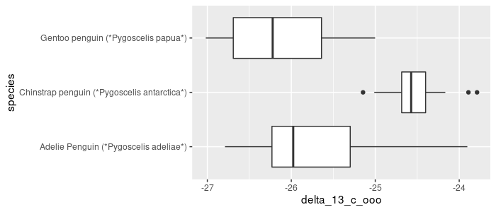
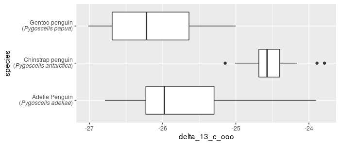
Make a sideways boxplot comparing δ13C (‰) across species. Rotate the graph to better display the labels:
pg_df %>%
  ggplot(aes(x = species, y = delta_13_c_ooo)) +
  geom_boxplot() +
  coord_flip()

Formatting the entire label is possible by modifying a theme element:
pg_df %>%
  ggplot(aes(x = species, y = delta_13_c_ooo)) +
  geom_boxplot() +
  coord_flip() +
  theme(axis.text.y = element_text(face = "italic"))

However, until recently, italicizing only the Latin name was much less straightforward.
ggtext allows for using (limited) markdown syntax within the plot labels. This functionality will soon be in ggplot2 but for now install and load ggtext.
# devtools::install_github("wilkelab/ggtext")
library(ggtext)
Remember markdown syntax?
pg_df %>%
  mutate(species = glue("{common} (*{latin}*)")) %>%
  ggplot(aes(x = species, y = delta_13_c_ooo)) +
  geom_boxplot() +
  coord_flip()
In order to apply the formatting, specify that this theme element should be interpreted as markdown. Recall that the X and Y axes are flipped!
pg_df %>%
  mutate(species = glue("{common} (*{latin}*)")) %>%
  ggplot(aes(x = species, y = delta_13_c_ooo)) +
  geom_boxplot() + coord_flip() +
  theme(axis.text.y = element_markdown())

The other html/markdown styles that can be interpreted are: line break, italics, bold, colors, fonts, super/subscript, and images.
pg_df %>%
  mutate(species = glue("{common}<br>(*{latin}*)")) %>%
  ggplot(aes(x = species, y = delta_13_c_ooo)) +
  geom_boxplot() + coord_flip() +
  theme(axis.text.y = element_markdown())
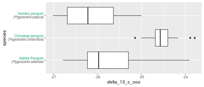
Because there is no markdown syntax for font color, html syntax is required to change font color:
pg_df %>%
  mutate(species = glue("<span style='color:#009E73'>{common}</span><br>(*{latin}*)")) %>%
  ggplot(aes(x = species, y = delta_13_c_ooo)) +
  geom_boxplot() + coord_flip() +
  theme(axis.text.y = element_markdown())
Explore color codes using the scales package, which underlies many other functions you may be using in ggplot figures already.
library(scales)
> show_col(viridis_pal()(3))

> show_col(brewer_pal(type = "qual", palette = "Dark2")(3))

In order to use a different color for each penguin species, we will add a new column to the data frame with the color hex code for each using a series of conditional statements with dplyr’s case_when function.
case_when(LHS ~ RHS, ...)
This will create a new vector of Right Hand Side (RHS) values based on whether cases evaluate to TRUE with the Left Hand Side (LHS). It can be handy for the purpose of labeling different classes of a continuous variable such as:
case_when(
  x < 10 ~ "small",
  x >= 10 & x < 20 ~ "medium",
  x >= 20 ~ "large")
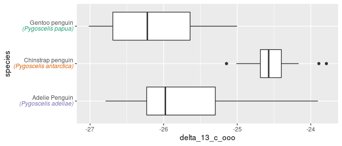
Add in the colors we identified from the Dark2 palette in a new column called color, using conditional statements to filter rows for each penguin species. Use color hex codes as the replacement value.
pg_df <- pg_df %>%
  mutate(color = case_when(common == "Gentoo penguin" ~ "#1B9E77",
                           common == "Chinstrap penguin" ~ "#D95F02",
                           common == "Adelie Penguin" ~ "#7570B3"))
The arguments to case_when are evaluated in order, so it is advised to list them from most specific to most general. If there were rows with other or NA values for the common name, we could designate what goes in the color column for those rows by adding a last conditional such as TRUE ~ "#000000".
Then use glue to include the species-specific color value in the axis label.
pg_df %>%
  mutate(species = glue("{common}<br><i style='color:{color}'>({latin})</i>")) %>%
  ggplot(aes(x = species, y = delta_13_c_ooo)) +
  geom_boxplot() + coord_flip() +
  theme(axis.text.y = element_markdown())
Categorical data
R has a special data type for handling categorial data called factors. Because they had a reputation for causing trouble…
> default.stringsAsFactors()
[1] FALSE
😲 this setting is new in R version 4 !!
Although read_csv had always defaulted strings to character data, there are situations where you may want to use factors, especially for modeling and plots – essentially whenever you want character vectors to not be alphabetical. forcats is intended to make this easier.
Species common names are in a character vector.
> class(pg_df$common)
[1] "character"
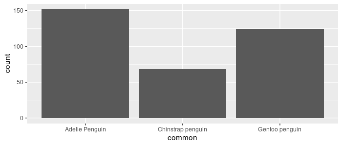
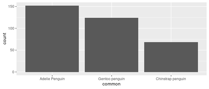
Controlling the order in which the 3 species appear in a plot is done with factors. If the data are kept as characters, plots will be sorted alphabetically (i.e. the default ordering for factor levels in base R).
> as.factor(pg_df$common) %>% levels()
[1] "Adelie Penguin" "Chinstrap penguin" "Gentoo penguin"
pg_df %>%
  ggplot(aes(x = common)) +
  geom_bar()
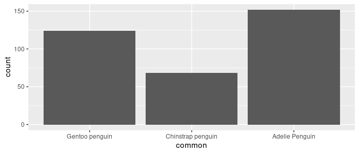
forcats::as_factor uses instead the order in which the levels appear in your data:
> as_factor(pg_df$common) %>% levels()
[1] "Gentoo penguin" "Chinstrap penguin" "Adelie Penguin"
Convert common into a factor and remake the same bar plot. Notice the ordering of the bars compared to the previous graph.
pg_df <- pg_df %>%
  mutate(common = as_factor(common))

pg_df %>%
  ggplot(aes(x = common)) +
  geom_bar()
Use fct_infreq to order the levels by how frequently they appear in the dataset.
pg_df %>%
  mutate(common = fct_infreq(common)) %>%
  ggplot(aes(x = common)) +
  geom_bar()
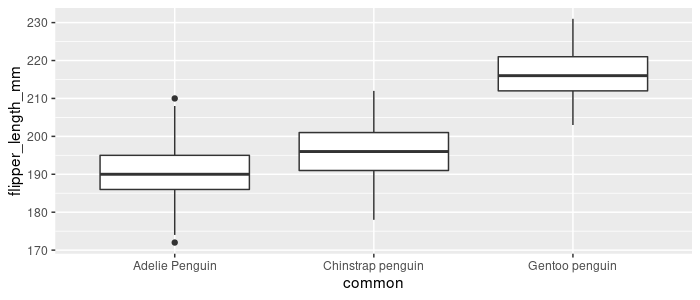
Or more generally, fct_reorder to use a function(.fun) of a different variable (.x). Order common by each level’s median flipper_length_mm:
pg_df %>%
  mutate(common = fct_reorder(common,
    .x = flipper_length_mm, .fun = median, na.rm = TRUE)) %>%
  ggplot(aes(x = common, y = flipper_length_mm)) +
  geom_boxplot()
All combinations of variables
To create a table with combinations of variables, use expand from the tidyr package. For example:
> pg_df %>% expand(island, sex, common)
# A tibble: 27 × 3
   island sex    common
   <chr>  <chr>  <fct>
 1 Biscoe FEMALE Gentoo penguin
 2 Biscoe FEMALE Chinstrap penguin
 3 Biscoe FEMALE Adelie Penguin
 4 Biscoe MALE   Gentoo penguin
 5 Biscoe MALE   Chinstrap penguin
 6 Biscoe MALE   Adelie Penguin
 7 Biscoe <NA>   Gentoo penguin
 8 Biscoe <NA>   Chinstrap penguin
 9 Biscoe <NA>   Adelie Penguin
10 Dream  FEMALE Gentoo penguin
# … with 17 more rows
To only include the combinations of variables that do appear in your data, put the column names inside of the nesting helper function.
pars <- pg_df %>% expand(nesting(island, sex, common))
> str(pars)
tibble [13 × 3] (S3: tbl_df/tbl/data.frame)
 $ island: chr [1:13] "Biscoe" "Biscoe" "Biscoe" "Biscoe" ...
 $ sex   : chr [1:13] "FEMALE" "FEMALE" "MALE" "MALE" ...
 $ common: Factor w/ 3 levels "Gentoo penguin",..: 1 3 1 3 1 2 3 2 3 3 ...
Summary
As you have seen, some core principles of the tidyverse
- Packages are united by common design structures so they work together (e.g. tidy evaluation)
- Functions emphasize modularity so you can break complex problems into small parts
- Functions emphasize consistency so you can easily expect what they will return
- Designed to write code that is easy to read and interpret
These are some of the cool functions we learned about
| Function | Package | Usage | Base R version |
|---|---|---|---|
map & friends |
purrr | iterate over objects | sapply, lapply |
glue |
glue | combining strings | paste0 |
case_when |
dplyr | if else | if else |
dir_ls |
fs | list files in a directory | list.files |
spec_csv |
readr | column specification | ? |
rename_with |
dplyr | use a function to rename columns | ? |
mdy & friends |
lubridate | smart date guessing | as.Date |
element_markdown() |
ggplot2 | plot text formatting | ? |
show_col |
scales | display colors | ? |
fct_reorder |
forcats | reorder factors | levels, reorder |
expand & friends |
tidyr | generate variable combinations | expand.grid |
Some other topics about the tidyverse that are worth looking into but we didn’t cover here:
- tidymodels - A framework for modeling and machine learning using tidy principles, including a website with extensive resources to learn about creating and tuning models. broom installs with tidyverse and is helpful for tidying up output from commonly used models such as
lmorcor.test - Deeper into rlang - To learn more about using tidy evaluation in functions, refer to this dplyr vignette, the documentation and cheatsheet for rlang, or one of these videos from the tidyverse developers.
- Functions in purrr to manipulate lists, and list columns in tibble data frames that can be nested and unnested
- Interval, period and duration classes in lubridate, for working with specific time spans. See the cheatsheet for examples of irregularities and inconsistencies that can complicate analyses with dates and times (e.g. leap years, daylight savings time, etc.).
Exercises
Exercise 1
Instead of returning an output of a specific type, the walk functions in purrr carry out a side effect (like displaying or saving a plot) without returning an object to your environment. Read about map variants that take multiple inputs, then use an appropriate function to save separate csv files for data about penguins from each of the studied islands using a list of data frames and a vector of filenames.
Hint: Check out the base split or dplyr group_split function for creating a list of data frames.
Exercise 2
Check out some specialized functions in fs for extracting parts of filepaths.
Remove "data/penguins/" and ".csv" from the filename strings using only functions in fs.
Exercise 3
The following vector dates represents 3 periods of time. Convert it into a list of 3 separate date vectors each split into the start and end dates of each period.
> dates <- c("2007-12-03 to 2009-12-01",
+            "2007 November 30 to 2009 October",
+            "1999 to 2010")
Hint: check out the truncation argument in ymd.
Exercise 4
Also use the different colors for each species within the plot geometry layer.
Hint: You will need a scale_ function
Exercise 5
Convert all character columns except for “comment” to factors using one mutate function.
Hint: Check out the across function
Exericse 6
Expand the pars data frame with a column of 10 model names for each of the unique combinations of island, sex, and species that appear in the data set. (should result in a 4 x 130 data frame)
Bonus Challenge
Use different images (such as from phylopic.org) to include in the labels representing each penguin species.
Solutions
Solution 1
> filenames <- glue::glue("{unique(pg_df$island)}.csv")
> pg_df %>%
+   dplyr::group_split(island) %>%
+   walk2(filenames, ~write_csv(.x, .y))
Solution 2
> pg_df$filename %>%
+   fs::path_ext_remove() %>%
+   fs::path_file()
Solution 3
> dates %>%
+   str_split("to", n = 2) %>%
+   map(~str_trim(.x)) %>% # or split on " to " for trimming whitespace
+   map(~ymd(.x, truncated = 2))
Solution 4
> pg_df %>%
+   mutate(species = glue("{common}<br><i style='color:{color}'>({latin})</i>")) %>%
+   ggplot(aes(x = species, y = delta_13_c_ooo)) +
+   geom_boxplot(aes(fill = color), alpha = 0.75) +
+   scale_fill_identity() + # tricky!
+   coord_flip() +
+   theme(axis.text.y = element_markdown())
Solution 5
> pg_df %>%
+   mutate(across(where(is.character) & !contains("comment"), as_factor))
Solution 6
> library(magrittr)
> model_names <- glue("model_{letters[1:10]}")
> pars %<>% crossing(model_names)
Solution 7
You’re on your own so far!
If you need to catch-up before a section of code will work, just squish it's 🍅 to copy code above it into your clipboard. Then paste into your interpreter's console, run, and you'll be ready to start in on that section. Code copied by both 🍅 and 📋 will also appear below, where you can edit first, and then copy, paste, and run again.
# Nothing here yet!