Basic Python

Lesson Objectives

• Earn your Python “learner’s permit”
• Work with Pandas, the DataFrame package
• Recognize differences between R and Python
• Hit the Autobahn with Scikit-learn

Specific Achievements

• Differentiate between data types and structures
• Learn to use indentation as syntax
• Import data and try a simple “split-apply-combine”
• Implement a SVM for binary classification

Why learn Python? While much of the academic research community has dived into R for an open source toolbox for data science, there are plenty of reasons to learn Python too. Some find they can learn to write scripts more quickly in Python, others find its object orientation a real boon. This lesson works towards a simple “machine learning” problem, which has long been a speciality of Python’s Scikit-learn package.

Machine Learning

Machine Learning is another take on regression (for continuous response) and classification (for categorical response).

• Emphasis on prediction over parameter inference
• Equal emphasis on probabilistic and non-probabilistic methods: whatever works
• Not necessarilly “supervised” (e.g. clustering)

This lesson will step through a non-probabilistic classifier, because it’s at far end of the spectrum relative to generalized linear regression. Some classification methods have probabilistic interpretations: logistic regression is actually a classifier, whether or not you follow through to choosing the most likely outcome or are satisfied with estimating its probability. Others optimize the classifier based on other abstract quantities: SVMs maximize the distance between the “support vectors”.

Jupyter

Sign into JupyterHub and open up worksheet.ipynb. This worksheet is an Jupyter Notebook document: it is divided into “cells” that are run independently but access the same Python interpreter. Use the Notebook to write and annotate code.

After opening worksheet.ipynb, right click anywhere in your notebook and choose “Create Console for Notebook”. Drag-and-drop the tabs into whatever arrangement you like.

Variables

Variable assignment attaches the label left of an = to the return value of the expression on its right.

a = 'xyz'
a

'xyz'

Colloquially, you might say the new variable a equals 'xyz', but Python makes it easy to “go deeper”. There can be only one string 'xyz', so the Python interpreter makes a into another label for the same 'xyz', which we can verify by id().

The “in-memory” location of a returned by id() …

> id(a)

738014016

… is equal to that of xyz itself:

> id('xyz')

738014016

The idiom to test this “sameness” is typical of the Python language: it uses plain English when words will suffice.

> a is 'xyz'

True

Equal but not the Same

The id() function helps demonstrate that “equal” is not the “same”.

b = [1, 2, 3]
id(b)

739311176

> id([1, 2, 3])

739310920

Even though b == [1, 2, 3] returns True, these are not the same object:

> b is [1, 2, 3]

False

Side-effects

The reason to be aware of what b is has to do with “side-effects”, an very import part of Python programming. A side-effect occurs when an expression generates some ripples other than its return value.

> b.pop()

3

> b

[1, 2]

Python is an object-oriented language from the ground up—everything is an “object” with some state to be more or less aware of. And side-effects don’t touch the label, they effect what the label is assigned to (i.e. what it is).

Question

Re-check the “in-memory” location—is it the same b?

Answer

Yes! The list got shorter but it is the same list.

Side-effects trip up Python programmers when an object has multiple labels, which is not so unusual:

c = b
b.pop()

2

> c

[1]

The assignment to c does not create a new list, so the side-effect of popping off the tail of b ripples into c.

A common mistake for those coming to Python from R, is to write b = b.append(4), which overwrites b with the value None that happens to be returned by the append() method.

Data Types

The basic data types are

Any object can be queried with type()

type('x')

<class 'str'>

Operators

Python supports the usual (or not) arithmetic operators for numeric types:

One or both of these might be a surprise:

5 ** 2

25

2 // 3

0

Some operators have natural extensions to non-numeric types:

a * 2

'xyzxyz'

Comparison operators are symbols or plain english:

Data Structures

The built-in structures for holding multiple values are:

• Tuple
• List
• Set
• Dictionary

Tuple

The simplest kind of sequence, a tuple is declared with comma-separated values, optionally inside (...). The tuple is a common type of return value for functions with multiple outputs.

T = 'x', 3, True
type(T)

<class 'tuple'>

To declare a one-tuple without (...), a trailing “,” is required.

T = 'cat',
type(T)

<class 'tuple'>

List

The more common kind of sequence in Python is the list, which is declared with comma-separated values inside [...]. Unlike a tuple, a list is mutable.

L = [3.14, 'xyz', T]
type(L)

<class 'list'>

Subsetting Tuples and Lists

Subsetting elements from a tuple or list is performed with square brackets in both cases, and selects elements using their integer position starting from zero—their “index”.

> L[0]

3.14

Negative indices are allowed, and refer to the reverse ordering: -1 is the last item in the list, -2 the second-to-last item, and so on.

> L[-1]

('cat',)

The syntax L[i:j] selects a sub-list starting with the element at index i and ending with the element at index j - 1.

> L[0:2]

[3.14, 'xyz']

A blank space before or after the “:” indicates the start or end of the list, respectively. For example, the previous example could have been written L[:2].

A potentially useful trick to remember the list subsetting rules in Python is to picture the indices as “dividers” between list elements.

 0      1       2          3 
 | 3.14 | 'xyz' | ('cat',) |
-3     -2      -1

Positive indices are written at the top and negative indices at the bottom. L[i] returns the element to the right of i whereas L[i:j] returns elements between i and j.

Set

The third and last “sequence” data structure is a set, useful for operations like “union” and “difference”. Declare a set with comma-separated values inside {...} or by casting another sequence with set().

S1 = set(L)
S2 = {3.14, 'z'}
S1.difference(S2)

{'xyz', ('cat',)}

Python is a rather principled language: a set is technically unordered, so its elements do not have an index. You cannot subset a set using [...].

Dictionary

Lists are useful when you need to access elements by their position in a sequence. In contrast, a dictionary is needed to find values based on arbitrary identifiers, called “keys”.

Construct a dictionary with comma-separated key: value pairs within {...}.

user = {
  'First Name': 'J.',
  'Last Name': 'Doe',
  'Email': 'j.doe@gmail.com',
}
type(user)

<class 'dict'>

Individual values are accessed using square brackets, as for lists, but the key must be used rather than an index.

user['Email']

'j.doe@gmail.com'

To add a single new element to the dictionary, define a new key:value pair by assigning a value to a novel key in the dictionary.

user['Age'] = 42

Dictionary keys are unique. Assigning a value to an existing key overwrites its previous value. You would replace the current Gmail address with user['Email'] = doedoe1337@aol.com.

Flow Control

The syntax for “if … then” tests and for-loops involves plain English and few special characters—you will easily ingest it. Whitespace actually serves as the most important special character, although you may not think of it that way, and that is our main motivation for looking at flow control.

For-loops

A for loop takes any “iterable” object and executes a block of code once for each element in the object.

squares = []
for i in range(1, 5):
    j = i ** 2
    squares.append(j)
len(squares)

4

The range(i, j) function creates an object that iterates from i up through j - 1; just like in the case of list slices, the range is not inclusive of the upper bound.

Indentation

Note the pattern of the block above:

• the for x in y expression is followed by a :
• the following lines are indented equally
• un-indenting indicates the end of the block

Compared with other programming languages in which code indentation only serves to enhance readability, Python uses indentation to define “code blocks”. In a sense, indentation serves two purposes in Python, enhancing readiblity and defining complete statements, which is kinda how we use indentation too.

Nesting Indentation

Each level of indentation indicates blocks within blocks. Nesting a conditional within a for-loop is a common case.

The following example creates a contact list (as a list of dictionaries), then performs a loop over all contacts. Within the loop, a conditional statement (if) checks if the name is ‘Alice’. If so, the interpreter prints her email address; otherwise it prints an empty string.

users = [
    {'Name':'Alice', 'Email':'alice@email.com'},
    {'Name':'Bob', 'Email': 'bob@email.com'},
    ]
for u in users:
    if u['Name'] == 'Alice':
        print(u['Email'])
    else:
        print('')

alice@email.com

Methods

The period is a special character in Python that accesses an object’s attributes and methods. In either the Jupyter Notebook or Console, typing an object’s name followed by . and then pressing the TAB key brings up suggestions.

squares.index(4)

1

We call this index() function a method of lists (recall that squares is of type 'list'). A useful feature of having methods attached to objects is that their documentation is attached too.

> help(squares.index)

Help on built-in function index:

index(...) method of builtins.list instance
    L.index(value, [start, [stop]]) -> integer -- return first index of value.
    Raises ValueError if the value is not present.

A major differnce between Python and R has to do with the process for making functions behave differently for different objects. In Python, a function is attached to an object as a “method”, while in R it is common for a “dispatcher” to examine the attributes of a function call’s arguments and chooses the particular function to use.

Dictionary’s have an update() method, for merging the contents of a second dictionary into the one calling update().

user.update({
  'Nickname': 'Jamie',
  'Age': 24,
})
user

{'First Name': 'J.', 'Last Name': 'Doe', 'Email': 'j.doe@gmail.com', 'Age': 24, 'Nickname': 'Jamie'}

Note a couple “Pythonic” style choices in the above:

1. Leave a space after the : when declaring key: value pairs
2. Trailing null arguments are syntactically correct, even advantageous
3. White space within (...) has no meaning and can improve readiability

The “style-guide” for Python scripting, PEP 8, is first authored by the inventor of Python and adhered too by many. It’s sometimes nice to know their is a preferred way of writing code, but don’t let it be a burden.

Pandas

If you have used the statistical programming language R, you are familiar with “data frames”, two-dimensional data structures where each column can hold a different type of data, as in a spreadsheet.

The analagous data frame package for Python is pandas, which provides a DataFrame object type with methods to subset, filter reshape and aggregate tabular data.

After importing pandas, we call its read_csv function to load the County Business Patterns (CBP) dataset.

import pandas as pd
cbp = pd.read_csv('data/cbp15co.csv')
cbp.dtypes

FIPSTATE     int64
FIPSCTY      int64
NAICS       object
EMPFLAG     object
EMP_NF      object
EMP          int64
QP1_NF      object
QP1          int64
AP_NF       object
AP           int64
EST          int64
N1_4         int64
N5_9         int64
N10_19       int64
N20_49       int64
N50_99       int64
N100_249     int64
N250_499     int64
N500_999     int64
N1000        int64
N1000_1      int64
N1000_2      int64
N1000_3      int64
N1000_4      int64
CENSTATE     int64
CENCTY       int64
dtype: object

As is common with CSV files, the inferred data types were not quite right.

cbp = pd.read_csv(
    'data/cbp15co.csv',
    dtype={'FIPSTATE':'str', 'FIPSCTY':'str'},
    )
cbp.dtypes

FIPSTATE    object
FIPSCTY     object
NAICS       object
EMPFLAG     object
EMP_NF      object
EMP          int64
QP1_NF      object
QP1          int64
AP_NF       object
AP           int64
EST          int64
N1_4         int64
N5_9         int64
N10_19       int64
N20_49       int64
N50_99       int64
N100_249     int64
N250_499     int64
N500_999     int64
N1000        int64
N1000_1      int64
N1000_2      int64
N1000_3      int64
N1000_4      int64
CENSTATE     int64
CENCTY       int64
dtype: object

There are many ways to slice a DataFrame. To select a subset of rows and/or columns by name, use the loc attribute and [ for indexing.

cbp.loc[:, ['FIPSTATE', 'NAICS']]

        FIPSTATE   NAICS
0             01  ------
1             01  11----
2             01  113///
3             01  1133//
4             01  11331/
...          ...     ...
2126596       56  812990
2126597       56  813///
2126598       56  8133//
2126599       56  81331/
2126600       56  813312

[2126601 rows x 2 columns]

As with lists, : by itself indicates all the rows (or columns). Unlike lists, the loc attribute returns both endpoints of a slice.

cbp.loc[2:4, 'FIPSTATE':'NAICS']

  FIPSTATE FIPSCTY   NAICS
2       01     001  113///
3       01     001  1133//
4       01     001  11331/

Use the iloc attribute of a DataFrame to get rows and/or columns by position, which behaves identically to list indexing.

cbp.iloc[2:4, 0:3]

  FIPSTATE FIPSCTY   NAICS
2       01     001  113///
3       01     001  1133//

The default indexing for a DataFrame, without using the loc or iloc attributes, is by column name.

cbp[['NAICS', 'AP']].head()

    NAICS      AP
0  ------  321433
1  11----    3566
2  113///    3551
3  1133//    3551
4  11331/    3551

The loc attribute also allows logical indexing, i.e. the use of a boolean array of appropriate length for the selected dimension. The subset of cbp with sector level NAICS codes can indexed with string matching.

logical_idx = cbp['NAICS'].str.match('[0-9]{2}----')
cbp = cbp.loc[logical_idx]
cbp.head()

   FIPSTATE FIPSCTY   NAICS EMPFLAG  ... N1000_3  N1000_4 CENSTATE  CENCTY
1        01     001  11----     NaN  ...       0        0       63       1
10       01     001  21----     NaN  ...       0        0       63       1
17       01     001  22----     NaN  ...       0        0       63       1
27       01     001  23----     NaN  ...       0        0       63       1
93       01     001  31----     NaN  ...       0        0       63       1

[5 rows x 26 columns]

Creation of new variables, our old favorite the full FIPS identifier, is done by assignment to new column names, using another str method.

cbp['FIPS'] = cbp['FIPSTATE'].str.cat(cbp['FIPSCTY'])
cbp.head()

   FIPSTATE FIPSCTY   NAICS EMPFLAG  ... N1000_4  CENSTATE CENCTY   FIPS
1        01     001  11----     NaN  ...       0        63      1  01001
10       01     001  21----     NaN  ...       0        63      1  01001
17       01     001  22----     NaN  ...       0        63      1  01001
27       01     001  23----     NaN  ...       0        63      1  01001
93       01     001  31----     NaN  ...       0        63      1  01001

[5 rows x 27 columns]

Index

The DataFrame object includes the notion of “primary keys” for a table in its Index construct. One or more columns that uniquely identify rows can be set aside from the remaining columns.

cbp = cbp.set_index(['FIPS', 'NAICS'])
cbp.head()

             FIPSTATE FIPSCTY EMPFLAG  ... N1000_4  CENSTATE CENCTY
FIPS  NAICS                            ...                         
01001 11----       01     001     NaN  ...       0        63      1
      21----       01     001     NaN  ...       0        63      1
      22----       01     001     NaN  ...       0        63      1
      23----       01     001     NaN  ...       0        63      1
      31----       01     001     NaN  ...       0        63      1

[5 rows x 25 columns]

Any hierarchical index can be “unstacked”, and all columns appropriately spread into a “wide” table layout.

cbp = cbp[['EMP', 'AP']].unstack(fill_value=0)

The last transformation kept only two variables for each FIPS and NAICS combination: the number of employees and the annual payroll (x $1000). By now, it may be obvious we are slowly working towards some goal!

The number of employees in just two sectors will serve as the set of variables (i.e. columns) by which we attempt to classify each county as “Metro” (i.e. urban) or not (i.e. rural). The first code is for Agriculture, Forestry, Fishing, and Hunting. The second is Accommodation and Food Services.

employment = cbp['EMP']
employment = employment.loc[:, ['11----', '72----']]
employment.head()

NAICS  11----  72----
FIPS                 
01001      70    2091
01003      14   12081
01005     180     594
01007      70     306
01009      10     679

Classification

The CBP dataset provides economic attributes of the three thousand and some US counties. The employment numbers are continuous attributes, and we expect those are somehow different between urban and rural counties.

We need a classifier suitable for:

1. many continuous “predictors”
2. a binary “response”

Continuous attributes paried with a binary class, which we hope to predict given a model and a set of training data, could be a problem for logistic regression. An alternative method, and a foundation of machine learning, is the Support Vector Machine.

Image by Alisneaky / CC BY-SA

The name arises from the main optimization task: choosing a subset of the training data attributes to be the “support vectors” (vector is another way of referring to a point in attribute space). The support vectors sit near (“support”) a barrier that more or less divides attribute space into regions dominated by a single class. The points sitting on the dashed lines above are the support vectors.

The USDA ERS classifies the counties of the US with a set of 9 Rural-Urban Continuum Codes. Joining these to the CBP attributes, and creating a binary “Metropolitan” class based on the the codes for urban-influenced areas, completes our dataset.

rural_urban = pd.read_csv(
    'data/ruralurbancodes2013.csv',
    dtype={'FIPS':'str'},
    ).set_index('FIPS')
rural_urban['Metro'] = rural_urban['RUCC_2013'] < 4

By default, the join will take place on the index, which serves as a primary key, for each table. It is a one-to-one join.

employment_rural_urban = employment.join(
    rural_urban['Metro'],
    how='inner',
    )

Only the single variable “Metro” is taken from the rural_urban table for use in the classification problem.

Model evaluation for SVMs and other machine learning methods lacking a probabilistic interpretion is based on subsetting data into “training” and “validation” sets.

import numpy as np

train = employment_rural_urban.sample(
    frac=0.5,
    random_state = np.random.seed(345))

Import the learning machine from sklearn, and pass the training data separately as the attributes (as X below) and class (as y).

from sklearn import svm
ml = svm.LinearSVC()

X = train.drop('Metro', axis=1).values[:, :2]
X = np.log(1 + X)
y = train['Metro'].values.astype(int)

ml.fit(X, y)

LinearSVC()

C:\Users\qread\AppData\Local\r-miniconda\envs\r-reticulate\lib\site-packages\sklearn\svm\_base.py:977: ConvergenceWarning: Liblinear failed to converge, increase the number of iterations.
  "the number of iterations.", ConvergenceWarning)

Why np.log(1 + X)? Remember, “whatever it takes” is the machine learning mantra. In this case the high skew of the employment numbers had attributes widely dispersed in attribute space, and the fit was worse (and harder to visualize). The offset with a positive number is necessary to keep counties with 0 employees in a sector.

Classifier Evaluation

The “confusion matrix” shows the largest numbers are on the diagonal—that is the number of metro and Non-metro data points correctly separated by the chosen support vectors.

from sklearn import metrics

metrics.confusion_matrix(y, ml.predict(X), (True, False))

array([[355, 238],
       [109, 869]], dtype=int64)

C:\Users\qread\AppData\Local\r-miniconda\envs\r-reticulate\lib\site-packages\sklearn\utils\validation.py:71: FutureWarning: Pass labels=(True, False) as keyword args. From version 0.25 passing these as positional arguments will result in an error
  FutureWarning)

A quick visualization using the mlxtend package shows the challenge of separating this attribute space!

from mlxtend.plotting import plot_decision_regions

plot_decision_regions(X, y, clf=ml, legend=2)

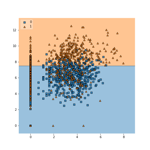
Kernel Method

The LinearSVM is rarely used in practice despite its speed—rare is the case when a hyperplane cleanly separates the attributes. The more general SVC machine accepts multiple kernel options that provide great flexibility in the shape of the barrier (no longer a hyperplane).

ml = svm.SVC(kernel = 'rbf', C=1, gamma='auto')
ml.fit(X, y)

SVC(C=1, gamma='auto')

The improvement in the confusion matrix is slight—we have not tuned the gamma value, which is automatically chosen based on the size of the dataset.

metrics.confusion_matrix(y, ml.predict(X), (True, False))

array([[322, 271],
       [ 35, 943]], dtype=int64)

C:\Users\qread\AppData\Local\r-miniconda\envs\r-reticulate\lib\site-packages\sklearn\utils\validation.py:71: FutureWarning: Pass labels=(True, False) as keyword args. From version 0.25 passing these as positional arguments will result in an error
  FutureWarning)

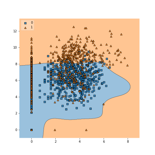
More important is to understand the nature of the separation, which can “wrap around” the attribute space as necessary.

plot_decision_regions(X, y, clf=ml, legend=2)

Summary

Python is said to have a gentle learning curve, but all new languages take practice.

Key concepts covered in this lesson include:

• Variables, or objects
• Data structures
• Methods
• pandas DataFrame
• Scikit-learn SVC

Additional critical packages for data science:

• matplotlib, plotly, seaborn for vizualization
• StatsModels, and pystan for model fitting
• PyQGIS, rasterio, Shapely, and Cartopy for GIS

Exercises

Exercise 1

Explore the use of in to test membership in a list. Create a list of multiple integers, and use in to test membership of some other numbers in your list.

View solution

Exercise 2

Based on what we have learned so far about lists and dictionaries, think up a data structure suitable for an address book of names and emails. Now create it! Enter the name and email address for yourself and your neighbor in a new variable called addr.

View solution

Exercise 3

Write a for-loop that prints all even numbers between 1 and 9. Use the modulo operator (%) to check for evenness: if i is even, then i % 2 returns 0, because % gives the remainder after division of the first number by the second.

View solution

Exercise 4

Tune the gamma parameter for the Support Vector Machine from above that used the rbf kernel method. It can take any postivie value. Can you improve the confusion matrix? How does gamma appear to affect the regions seen with plot_decision_regions? Does the consuion matrix look okay out-of-sample (i.e. making predictions for the counties not used for training)?

Solutions

Solution 1

answers = [2, 15, 42, 19]
42 in answers

Return

Solution 2

addr = [
  {'name': 'Alice', 'email': 'alice@gmail.com'},
  {'name': 'Bob', 'email': 'bob59@aol.com'},
]

Return

Solution 3

for i in range(1, 9):
  if i % 2 == 0:
    print(i)

Return