Bas(e|ic) R

Lesson 1 with Ian Carroll and Mary Shelly

Why learn R?
The Console
The Environment
The Editor
Data types
Multi-dimensional data structures
Load data into R
Parts of an Object
Base plotting
Functions
Flow control
Distributions and Statistics
Review
Exercise solutions

Why learn R?

High-level programming language good for interactive statistical analysis
General purpose programming language for scripting entire data-processing pipelines
Large selection of add-on packages that extend the capabilities of “base R”
Large user community especially within statistics and ecology
Open source

The Console

The interpreter accepts R commands interactively through the console. Basic math, as you would type it on a calculator, is usually a valid command in the R language:

1 + 2

[1] 3

5/3

[1] 1.666667

4^2

[1] 16

Question: Why is the output prefixed by [1]?
Answer: That’s the index, or position in a vector, of the first result.

A command giving a vector of results shows this clearly:

seq(1, 50)

 [1]  1  2  3  4  5  6  7  8  9 10 11 12 13 14 15 16 17 18 19 20 21 22 23
[24] 24 25 26 27 28 29 30 31 32 33 34 35 36 37 38 39 40 41 42 43 44 45 46
[47] 47 48 49 50

The interpreter understands more than arithmatic operations! The last command was to use (or “call”) the function seq(). Most of “learning R” involves getting to know a whole lot of functions, the effect of each function’s arguments (e.g. the input values 1 and 10), and what each function returns (e.g. the output vector).

Basic math

A good place to begin learning R functions is with its built-in mathematical functionality:

binary operators +, -, *, /, and ^ (for raising to a power)
tests of equality (“==”) and inequality (“<” and “>”)
“smooth” functions like sin, log, and sqrt
additional functions like max, range, and mean

Use binary operators by inserting them between two numbers, grouped by parentheses when necessary.

(1 + 2) / 3

[1] 1

Use functions by calling them with comma-separated arguments between parentheses.

logb(2, 2)

[1] 1

Exercise 1

The quadratic formula for the two values of $x$ that satisfy the equation $a x^2 + b x + c = 0$ is

$\frac{-b \pm \sqrt{b^2 - 4 a c}}{2 a}.$

Use the quadratic formula to calculate both values of $x$ that solve $1.5 x^2 + 0.3 x - 2.9 = 0$ .

View solution

Assignment

When you start a new session, the R interpreter already knows many things, including

any number
any string of characters
operators that are universal (e.g. + or /) and specific to R (e.g. $ or %*%)
functions in base R

To reference a number or function you just type it in as above. To referece a string of characters you must surround them in quotation marks.

'ab.cd'

[1] "ab.cd"

Without quotation marks, the interpreter checks for things named ab.cd and doesn’t find anything:

ab.cd

Error in eval(expr, envir, enclos): object 'ab.cd' not found

Question: Is it better to use ' or "?
Answer: Neither one is better. You will often encounter stylistic choices like this, so if you don’t have a personal preference try to mimic existing styles.

We can expand the vocabulary known to the R interpreter by creating a new variable. Using the symbol <- is referred to as assignment: we assign the output of any command to the right of <- to any variable written to its left.

x <- seq(1, 50)

You’ll notice that nothing prints to the console, because we assigned the output to a variable. We can print the value of x by evaluating it without assignment.

 [1]  1  2  3  4  5  6  7  8  9 10 11 12 13 14 15 16 17 18 19 20 21 22 23
[24] 24 25 26 27 28 29 30 31 32 33 34 35 36 37 38 39 40 41 42 43 44 45 46
[47] 47 48 49 50

Assigning values to new variables (to the left of a <-) is the only time you can reference something previously unknown to the interpreter. All other commands must reference things already in the interpreter’s vocabulary.

Once assigned to a variable, a value becomes known to R and you can refer to it in other commands.

y <- 'ab.cd'
typeof(y)

[1] "character"

Top of Section

The Environment

In the RStudio IDE, the environment tab displays the variables added to R’s vocabulary in the current session.

these variables do not persist between sessions (automatic saving and loading from a .RData file is discouraged)
existing variables only change their value on re-assignment

Top of Section

The Editor

The console is for evaluating commands you don’t intend to keep or reuse. It’s useful for testing commands and poking around. The editor is where you compose scripts that will process data, perform analyses, code up visualizations, and even write reports.

These work together in RStudio, which has multiple ways to send parts of the script you are editing to the console for immediate evaluation. Alternatively you can “source” the entire script.

Open up “worksheet-1.R” in the editor, and follow along by replacing the ... placeholders with the code here. Then evalute just this line (Ctrl+Enter on Windows, ⌘+Enter on Mac OS).

vals <- seq(1, 100)

Let’s review the elements of this statement, from left to right:

vals is the name of a (new) variable
<- is an operator that assigns what’s named on the left to equal the result of the expression on the right
seq is the name of the function
( is the opening paren of the function call
1 and 100 are both arguments, or parameters, to the function
) is the closing paren of a function call

Question: Why call vals a “variable” and seq a “function”?
Answer: It is true they are both names of objects known to R, and could be called variables. But seq has the important distinguishing feature of being callable, which is indicated in documentation by writing the function name with empty parens, as in seq().

Our call to the function seq could have been much more explicit. We could give the arguments by the names that seq is expecting.

vals <- seq(from = 1,
            to = 100)

Run this code either line-by-line, or highlight the section to run (optionally with keyboard shortcut Ctrl-Return or ⌘ Return).

Question: What’s an advantage of naming arguments?
Answer: One advantage is that you can put them in any order. A related advantage is that you can then skip some arguments, which is fine to do if each skipped argument has a default value. A third advantage is code readability, which you should always be concious of while writing in the editor.

Readability

Code readability in the editor cuts both ways: sometimes verbosity is useful, sometimes it is cumbersome. The seq() function has an operator form available when only the from and to arguments are needed.

1:100

  [1]   1   2   3   4   5   6   7   8   9  10  11  12  13  14  15  16  17
 [18]  18  19  20  21  22  23  24  25  26  27  28  29  30  31  32  33  34
 [35]  35  36  37  38  39  40  41  42  43  44  45  46  47  48  49  50  51
 [52]  52  53  54  55  56  57  58  59  60  61  62  63  64  65  66  67  68
 [69]  69  70  71  72  73  74  75  76  77  78  79  80  81  82  83  84  85
 [86]  86  87  88  89  90  91  92  93  94  95  96  97  98  99 100

The : operator should be used whenever possible because it replaces a common, cumbersome function call with an brief, intuitive syntax. Likewise, the assign function duplicates the functionallity of the <- symbol, but is never used when the simpler operator will suffice.

Function documentation

How would you get to know these properties and the names of a function’s arguments?

?seq

How would you even know what function to call?

??sequence

Top of Section

Data types

Type	Example
integer	-4, 0, 999
double	3.1, -4, Inf, NaN
character	‘a’, “4”, “👏”
logical	TRUE, FALSE
missing	NA

Data structures

Compound objects, built from one or more of these data types, or even other objects.

Common one-dimensional, array data structures:

Vectors
Lists
Factors

Vectors

Vectors are the basic data structure in R. They are a collection of data that are all of the same type. Create a vector by combining elements together using the function c(). Use the operator : for a sequence of numbers (forwards or backwards), otherwise separate elements with commas.

counts <- c(4, 3, 7, 5)

All elements of an vector must be the same type, so when you attempt to combine different types they will be coerced to the most flexible type.

c(1, 2, "c")

[1] "1" "2" "c"

Lists

Lists are like vectors but their elements can be of any data type or structure. You construct lists by using list() instead of c().

list(1, 2, "c")

[[1]]
[1] 1

[[2]]
[1] 2

[[3]]
[1] "c"

Lists can even include another list!

list(1, list(2, 3))

[[1]]
[1] 1

[[2]]
[[2]][[1]]
[1] 2

[[2]][[2]]
[1] 3

Exercise 2

Look at the outputs of list(1, list(2, 3)) and c(1, list(1, 2)). Store the output of each command as new variables, and then examine each variable’s structure with the str() function. What’s different about the structure of the two variables? Are both lists?

View solution

Factors

A factor is a vector that can contain only predefined values, and is used to store categorical data. Factors are built on top of integer vectors using two attributes: the class(), “factor”, which makes them behave differently from regular integer vectors, and their levels(), or the set of allowed values.

Use factor() to create a vector with predefined values, which are often characters or “strings”.

education <- factor(
    c("college", "highschool", "college", "middle"),
    levels = c("middle", "highschool", "college"))

str(education)

 Factor w/ 3 levels "middle","highschool",..: 3 2 3 1

A factor can be unorderd, as above, or ordered with each level somehow “less than” the next.

education <- factor(
    c("college", "highschool", "college", "middle"),
    levels = c("middle", "highschool", "college"),
    ordered = TRUE)

str(education)

 Ord.factor w/ 3 levels "middle"<"highschool"<..: 3 2 3 1

Top of Section

Multi-dimensional data structures

Data can be stored in several types of data structures depending on its complexity.

Dimensions	Homogeneous	Heterogeneous
1d	c()	list()
2d	matrix()	data.frame()
nd	array()

Of these, the data frame is far and away the most used.

Data frames

Data frames are 2-dimensional and can contain heterogenous data like numbers in one column and a factor in another.

It is the data structure most similar to a spreadsheet, with two key differences:

Data frames columns are equal-length vectors.
As vectors, the columns are homogeneous and cannot hold values of the wrong type.

Creating a data frame from scratch can be done by combining vectors with the data.frame() function.

df <- data.frame(education, counts)

df

   education counts
1    college      4
2 highschool      3
3    college      7
4     middle      5

Some functions to get to know your data frame are:

Function	Output
`dim()`	dimensions
`nrow()`	number of rows
`ncol()`	number of columns
`names()`	(column) names
`str()`	structure
`summary()`	summary info
`head()`	shows beginning rows

names(df)

[1] "education" "counts"

Exercise 3

Create a data frame with two columns, one called “species” and another called “abund”. Store your data frame as a variable called data. You can do this with or without populating the data frame with values.

View solution

Top of Section

Load data into R

We will use the function read.csv() that reads in a Comma-Separated-Values file by passing it the location of the file. The essential argument for the function to read in data is the path to the file, and optinal additional arguments specify additional ways of reading the data. Additional file types can be read in using read.table(); in fact, read.csv() is a simple wrapper for the read.table() function that specifies default values for some of the optional arguments.

Type a comma after read.csv( and then press tab to see what arguments that this function takes. Hovering over each item in the list will show a description of that argument from the help documentation about that function. Specify the values to use for an argument using the syntax name = value.

read.csv(file = "data/plots.csv", header = TRUE)

   id                 treatment
1   1         Spectab exclosure
2   2                   Control
3   3  Long-term Krat Exclosure
4   4                   Control
5   5          Rodent Exclosure
6   6 Short-term Krat Exclosure
7   7          Rodent Exclosure
8   8                   Control
9   9         Spectab exclosure
10 10          Rodent Exclosure
11 11                   Control
12 12                   Control
13 13 Short-term Krat Exclosure
14 14                   Control
15 15  Long-term Krat Exclosure
16 16          Rodent Exclosure
17 17                   Control
18 18 Short-term Krat Exclosure
19 19  Long-term Krat Exclosure
20 20 Short-term Krat Exclosure
21 21  Long-term Krat Exclosure
22 22                   Control
23 23          Rodent Exclosure
24 24          Rodent Exclosure

Question: Is the header argument necessary?
Answer: No. Look at ?read.csv to see that TRUE is the default value for this argument.

Use the assignment operator “<-“ to store that data in memory and work with it

plots <- read.csv(file = "data/plots.csv")
animals <- read.csv(file = "data/animals.csv")

You can specify what indicates missing data in the read.csv function using either na.strings = "NA" or na = "NA". You can also specify multiple things to be interpreted as missing values, such as na.strings = c("missing", "no data", "< 0.05 mg/L", "XX").

After reading in the “animals.csv” and “plots.csv” files, let’s explore what types of data are in each column and what kind of structure your data has.

str(plots)

'data.frame':	24 obs. of  2 variables:
 $ id       : int  1 2 3 4 5 6 7 8 9 10 ...
 $ treatment: Factor w/ 5 levels "Control","Long-term Krat Exclosure",..: 5 1 2 1 3 4 3 1 5 3 ...

summary(plots)

       id                            treatment
 Min.   : 1.00   Control                  :8  
 1st Qu.: 6.75   Long-term Krat Exclosure :4  
 Median :12.50   Rodent Exclosure         :6  
 Mean   :12.50   Short-term Krat Exclosure:4  
 3rd Qu.:18.25   Spectab exclosure        :2  
 Max.   :24.00

Exercise 4

By default, all character data is read in to a data.frame as factors. Use the read.csv() argument stringsAsFactors to suppress this behavior, then subsequently modify the sex column in animals to make it a factor. Columns of a data.frame are identified to the R interpreter with the $ operator, e.g. animals$sex. We’ll see more on this below.

View solution

Top of Section

Parts of an Object

Parts of objects are always accessible, either by their name or by their position, using square brackets: [ and ].

Position

counts[1]

[1] 4

counts[3]

[1] 7

Names

Parts of an object can usually also have a name. The names can be given when you are creating a vector or afterwards using the names() function.

df['education']

   education
1    college
2 highschool
3    college
4     middle

names(df) <- c('ed', 'ct')

df['ed']

          ed
1    college
2 highschool
3    college
4     middle

Question: This use of <- with names(x) on the left is a little odd. What’s going on?
Answer: We are overwriting an existing variable, but one that is accessed through the output of the function on the left rather than the global environment.

In a multi-dimensional array, you separate the dimension along which a part is requested with a comma.

df[3, 'ed']

[1] college
Levels: middle < highschool < college

It’s fine to mix names and indices when selecting parts of an object.

Subsetting ranges

There are multiple ways to simultaneously extract multiple parts of an object.

Use in brackets	Subset instructions
positive integers	elements at the specified positions
negative integers	omit elements at the specified positions
logical vectors	select elements where the corresponding value is TRUE
nothing	return the original vector (all)

days <- c("Sunday", "Monday", "Tuesday", "Wednesday", "Thursday", "Friday", "Saturday")
weekdays <- days[2:6]
weekend <- days[c(1, 7)]

weekdays

[1] "Monday"    "Tuesday"   "Wednesday" "Thursday"  "Friday"

weekend

[1] "Sunday"   "Saturday"

Exercise 5

Get weekdays using negative integers.
Get M-W-F using a call to seq() to specify the positions (don’t forget to ?seq).

View solution

Subsetting data frames

The $ sign is an operator that makes for quick access to a single, named part of an object. It’s most useful when used interactively with “tab completion” on the columns of a data frame.

df$ed

[1] college    highschool college    middle    
Levels: middle < highschool < college

A logical test applied to a single column produces a vector of TRUE and FALSE values that’s the right length for subsetting the data.

df[df$ed == 'college', ]

       ed ct
1 college  4
3 college  7

Exercise 6

Subset the data frame df by row position and column name such that you obtain the following output.

[1] highschool college
Levels: middle < highschool < college

View solution

Top of Section

Base plotting

R has excellent plotting capabilities for many types of graphics. The plot() function is the most basic plotting function, and uses the data provided to determine what kind of plot to make.

For more advanced plotting such as multi-faceted plots, the libraries lattice and ggplot2 are excellent options.

Scatterplots

Providing plots with separate “x” and “y” coordinates produces a scatterplot.

plot(animals$hindfoot_length, animals$weight)

plot of chunk unnamed-chunk-1

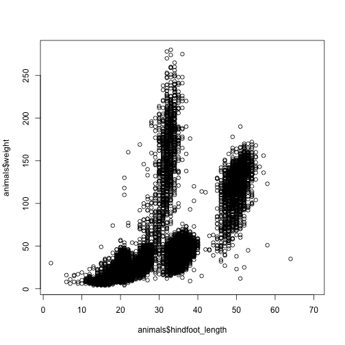
Using R’s formula notation, as in plot(weight ~ hindfoot_length, data = animals), is a more readable syntax for some.

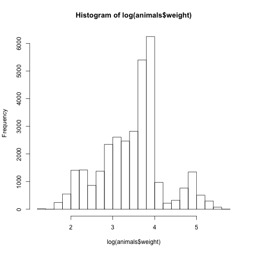
Histograms

To plot binned counts of a single variable, use the hist function.

hist(log(animals$weight))

plot of chunk unnamed-chunk-2

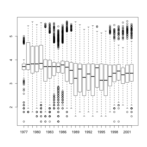
Boxplots

Use boxplot to compare the number of species seen each year.

boxplot(log(weight) ~ year, data = animals)

plot of chunk unnamed-chunk-3

Top of Section

Functions

The purpose of R functions is to package up a batch of commands. There are several reasons to develop functions

reuse
readability
modularity
consistency

Writing functions to use multiple times within a project prevents you from duplicating code, a real time-saver when you want to update what the function does. If you see blocks of similar lines of code through your project, those are usually candidates for being moved into functions.

Anatomy of a function

Writing functions is also a great way to understand the terminology and workings of R. Like all programming languages, R has keywords that are reserved for import activities, like creating functions. Keywords are usually very intuitive, the one we need is function.

function(...) {
    ...
    return(...)
}

Three components:

arguments: control how you can call the function
body: the code inside the function
return value: controls what output the function gives

We’ll make a function to extract the first row of its argument, which we give a name to use inside the function:

function(dat) {
    result <- dat[1, ]
    return(result)
}

Note that dat doesn’t exist until we call the function, which merely contains the instructions for how any dat will be handled.

Finally, we need to give the function a name so we can use it like we used c() and seq() above.

first <- function(dat) {
    result <- dat[1, ]
    return(result)
}

first(df)

       ed ct
1 college  4

Question: Can you explain the result of entering first(counts) into the console?
Answer: The function caused an error, which prompted the interpreter to print a helpful error message. Never ignore an error message. (It’s okay to ignore a “warning”.)

Top of Section

Flow control

The R interpreter’s “focus” flows through a script (or any section of code you run) line by line. Without additional instruction, every line is processed from the top to bottom. “Flow control” is the generic term for causing the interpreter to repeat or skip certain lines, using concepts like “for loops” and “if/else conditionals”.

Flow control happens within blocks of code isolated between curly braces { and }, known as “statements”.

if (...) {
    ...
} else {
    ...
}

The keyword if must be followed by a logical test which determines, at runtime, what to do next. The R interpreter goes to the first statement if the logical value is TRUE and to the second statement if it’s FALSE.

An if/else conditional would allow the first function to avoid the error thrown by calling first(counts).

first <- function(dat) {
    if (is.vector(dat)) {
        result <- dat[1]
    } else {
        result <- dat[1, ]
    }
    return(result)
}

first(df)

       ed ct
1 college  4

first(counts)

[1] 4

Exercise 7

The keywords else and if can be combined to allow flow control among more than two statements.

if (...) {
    ...
} else if {
    ...
} else if {
   ...
} else {
   ...
}

Expand the first function once again to differentiate between dat provided as a matrix and as a data.frame. It’s up to you what the “first” element of a matrix should be!

View solution

Top of Section

Distributions and Statistics

Since it is designed for statistics, R can easily draw random numbers from statistical distributions and calculate distribution values.

To generate random numbers from a normal distribution, use the function rnorm()

samp <- rnorm(n = 10)

samp

 [1] -0.78113282 -0.06103047 -1.15900799  0.26156262  0.46521782
 [6] -0.15671861  0.68824774 -1.26014231  1.05630340  2.86988207

Function	Returns	Notes
`rnorm()`	Draw random numbers from normal distribution	Specify `n`, `mean`, `sd`
`dnorm()`	Probability density at a given number
`pnorm()`	Cumulative probability up to a given number	left-tailed by default
`qnorm()`	The quantile given a cumulative probability	opposite of pnorm

Statistical distributions and their functions. See Table 14.1 in R for Everyone by Jared Lander for a full table.

Distribution	Functions
Normal	*norm
Binomial	*binom
Poisson	*pois
Gamma	*gamma
Exponential	*exp
Uniform	*unif
Logistic	*logis

R has built in functions for handling many statistical tests.

x <- rnorm(n = 100, mean = 25, sd = 7)
y <- rbinom(n = 100, size = 50, prob = .85)

t.test(x, y)


	Welch Two Sample t-test

data:  x and y
t = -22.664, df = 117.39, p-value < 2.2e-16
alternative hypothesis: true difference in means is not equal to 0
95 percent confidence interval:
 -19.54175 -16.40111
sample estimates:
mean of x mean of y 
 24.39857  42.37000

Linear regression with the lm() function uses a formula notation to specify relationships between variables (e.g. y ~ x).

fit <- lm(y ~ x)

summary(fit)


Call:
lm(formula = y ~ x)

Residuals:
    Min      1Q  Median      3Q     Max 
-5.3884 -1.3721 -0.3561  1.6289  5.6395 

Coefficients:
             Estimate Std. Error t value Pr(>|t|)    
(Intercept) 42.418347   0.789681  53.716   <2e-16 ***
x           -0.001982   0.030921  -0.064    0.949    
---
Signif. codes:  0 '***' 0.001 '**' 0.01 '*' 0.05 '.' 0.1 ' ' 1

Residual standard error: 2.333 on 98 degrees of freedom
Multiple R-squared:  4.19e-05,	Adjusted R-squared:  -0.01016 
F-statistic: 0.004107 on 1 and 98 DF,  p-value: 0.949

Exercise 8

Recall the formula notation used to plot hindfoot_length against weight for the observations in the animals data frame: plot(hindfoot_length ~ weight, data = animals). Instead of the plot function, use the lm function to estimate the coefficient of log(weight) as a predictor of log(hindfoot_length).

View solution

Top of Section

Review

In this introduction to R, we briefly touched on several key principle of scientific programming.

Data types
Assignment
Reading data
Subsetting data
Functions (keyword function)
Flow control (keywords if and else):
Plots
Statistics

Special characters in R

Perhaps more than most languages, an R script can appear like a jumble of archaic symbols. Here is a little table of characters to recognize as having special meaning

Symbol	Meaning
`.`
`?`	get help
`#`	comment
`:`	sequence
`::`, `:::`	access namespaces (advanced)
`<-`	assignment
`->`	assignment
`[ ]`	selection
`$`	selection
`% %`	infix operators, e.g. `%*%`
`{ }`	statements
`@`	slot (advanced)

Yes, the . in R has no fixed meaning and is often used as _ might be used to separate words in a variable name.

Top of Section

Exercise solutions

Solution 1

First solution:

(-0.3 + sqrt(0.3 ^ 2 - 4 * 1.5 * -2.9)) / (2 * 1.5)

[1] 1.294035

Second solution:

(-0.3 - sqrt(0.3 ^ 2 - 4 * 1.5 * -2.9)) / (2 * 1.5)

[1] -1.494035

Solution 2

x <- list(1, list(2, 3))
y <- c(1, list(2, 3))

str(x)

List of 2
 $ : num 1
 $ :List of 2
  ..$ : num 2
  ..$ : num 3

str(y)

List of 3
 $ : num 1
 $ : num 2
 $ : num 3

The variable x contains two elements, a number and a list. The variable y has concatenation of the two arguments, coerced to the more flexible of the two (a list is more flexible than a number). Both x and y are lists.

Solution 3

species <- c()
abund <- c()
data <- data.frame(species, abund)

str(data)

'data.frame':	0 obs. of  0 variables

Solution 4

animals <- read.csv('data/animals.csv', stringsAsFactors = FALSE, na.strings = '')
animals$sex <- factor(animals$sex)

str(animals)

'data.frame':	35549 obs. of  9 variables:
 $ id             : int  2 3 4 5 6 7 8 9 10 11 ...
 $ month          : int  7 7 7 7 7 7 7 7 7 7 ...
 $ day            : int  16 16 16 16 16 16 16 16 16 16 ...
 $ year           : int  1977 1977 1977 1977 1977 1977 1977 1977 1977 1977 ...
 $ plot_id        : int  3 2 7 3 1 2 1 1 6 5 ...
 $ species_id     : chr  "NL" "DM" "DM" "DM" ...
 $ sex            : Factor w/ 2 levels "F","M": 2 1 2 2 2 1 2 1 1 1 ...
 $ hindfoot_length: int  33 37 36 35 14 NA 37 34 20 53 ...
 $ weight         : int  NA NA NA NA NA NA NA NA NA NA ...

Solution 5

sol5a <- days[c(-1, -7)]
sol5b <- days[seq(2, 7, 2)]

sol5a

[1] "Monday"    "Tuesday"   "Wednesday" "Thursday"  "Friday"

sol5b

[1] "Monday"    "Wednesday" "Friday"

Solution 6

sol6 <- df[2:3, 'ed']

sol6

[1] highschool college   
Levels: middle < highschool < college

Solution 7

first <- function(dat) {
    if (is.vector(dat)) {
        result <- dat[1]
    } else if (is.matrix(dat)) {
        result <- dat[1, 1]
    } else {
        result <- dat[1, ]
    }
    return(result)
}

m <- matrix(1:9, nrow = 3, ncol = 3)
first(m)

[1] 1

Solution 8

animals.hl_model <- lm(log(hindfoot_length) ~ log(weight), data = animals)

coef(animals.hl_model)[2]

log(weight) 
  0.3961338

Top of Section

Bas(e|ic) R

Contents

Why learn R?

The Console

Basic math

Exercise 1

Assignment

The Environment

The Editor

Readability

Function documentation

Data types

Data structures

Vectors

Lists

Exercise 2

Factors

Multi-dimensional data structures

Data frames

Exercise 3

Load data into R

Exercise 4

Parts of an Object

Position

Names

Subsetting ranges

Exercise 5

Subsetting data frames

Exercise 6

Base plotting

Scatterplots

Histograms

Boxplots

Functions

Anatomy of a function

Flow control

Exercise 7

Distributions and Statistics

Exercise 8

Review

Special characters in R

Exercise solutions

Solution 1

Solution 2

Solution 3

Solution 4

Solution 5

Solution 6

Solution 7

Solution 8