Basic R
Handouts for this lesson need to be saved on your computer. Download and unzip this material into the directory (a.k.a. folder) where you plan to work.
Lesson Objectives
- Meet the R “Console”, “Editor”, and “Environment” within RStudio
- Understand that R “packages” extend it to the “bleeding-edge”
- Join a vast user community
within statistics and ecology - Learn what “free software” does for reproducible research
Specific Achievements
- Use R interactively for data exploration
- Create an R script for non-interactive data crunching
- Perform general purpose programming operations
What is R?
- Language: a vocabulary and a syntax (with lots of punctuation!)
- Interpreter: software that evaluates statements in the R language
Console
The interpreter accepts commands interactively through the console.
Basic math, as you would type it on a calculator, is usually a valid command in the R language:
> 1 + 2
[1] 3
> 4^2
[1] 16
- Question
- Why is the output prefixed by
[1]? - Answer
- That’s the index, or position in a vector, of the first result.
A command giving a vector of results shows this clearly:
> seq(1, 100)
  [1]   1   2   3   4   5   6   7   8   9  10  11  12  13  14  15  16  17  18
 [19]  19  20  21  22  23  24  25  26  27  28  29  30  31  32  33  34  35  36
 [37]  37  38  39  40  41  42  43  44  45  46  47  48  49  50  51  52  53  54
 [55]  55  56  57  58  59  60  61  62  63  64  65  66  67  68  69  70  71  72
 [73]  73  74  75  76  77  78  79  80  81  82  83  84  85  86  87  88  89  90
 [91]  91  92  93  94  95  96  97  98  99 100
The interpreter understands more than arithmatic operations.
That last command told it to use (or “call”) the function seq().
Most of “learning R” involves getting to know a whole lot of functions, the
effect of each function’s arguments (e.g. the input values 1 and 100), and
what each function returns (e.g. the output vector).
R as Calculator
A good place to begin learning R is with its built-in mathematical functionality.
Arithmatic Operators
Try +, -, *, /, and ^ (for raising to a power).
> 5/3
[1] 1.666667
Logical Tests
Test equality with == and inequality with <=, <, !=, >, or >=.
> 1/2 == 0.5
[1] TRUE
Math Functions
Common mathematical functions like sin, log, and sqrt, exist along side some universal constants.
> sin(2 * pi)
[1] -2.449294e-16
Generic Functions
Functions do more than math! Functions like ‘rep’, ‘sort’, and ‘range’ are pre-packaged instructions for processing user input.
> rep(2, 5)
[1] 2 2 2 2 2
Parentheses
Sandwiching something with ( and ) has two possible meanings.
Group sub-expressions by parentheses where needed.
> (1 + 2) / 3
[1] 1
Call functions by typing their name and comma-separated arguments between parentheses.
> logb(2, 2)
[1] 1
Environment
In the RStudio IDE, the environment tab displays any variables added to R’s vocabulary in the current session. In a brand new session, the R interpreter already recognizes many things, despite the environment being “empty”.
With an “empty” environment, the interpreter still recognizes:
- any number
- any string of characters
- nearly universal operators (e.g.
+and/) - operators specific to R (e.g.
$and%*%) - functions in “base R”
To reference a number or function just type it in as above. To referece a string of characters, surround them in quotation marks.
> 'ab.cd'
[1] "ab.cd"
Without quotation marks, the interpreter checks for things in the environment
named ab.cd and doesn’t find anything:
> ab.cd
Error in eval(expr, envir, enclos): object 'ab.cd' not found
- Question
- Is it better to use
'or"? - Answer
- Neither one is better. You will often encounter stylistic choices like this, so if you don’t have a personal preference try to mimic existing styles.
Assignment
You can expand the vocabulary known to the R interpreter by creating a new
variable. Using the symbol <- is referred to as assignment: the output of
any command to the right of <- gets the name given on its left.
> x <- seq(0, 100)
You’ll notice that nothing prints to the console, because we assigned the output
to a variable. We can print the value of x by evaluating it without
assignment.
> x
  [1]   0   1   2   3   4   5   6   7   8   9  10  11  12  13  14  15  16  17
 [19]  18  19  20  21  22  23  24  25  26  27  28  29  30  31  32  33  34  35
 [37]  36  37  38  39  40  41  42  43  44  45  46  47  48  49  50  51  52  53
 [55]  54  55  56  57  58  59  60  61  62  63  64  65  66  67  68  69  70  71
 [73]  72  73  74  75  76  77  78  79  80  81  82  83  84  85  86  87  88  89
 [91]  90  91  92  93  94  95  96  97  98  99 100
Assigning values to new variables (to the left of a <-) is the only time you
can reference something previously unknown to the interpreter. All other
commands must reference things already in the interpreter’s vocabulary.
Once assigned to a variable, a value becomes known to R and you can refer to it in other commands.
> plot(x, sin(x * 2 * pi / 100))
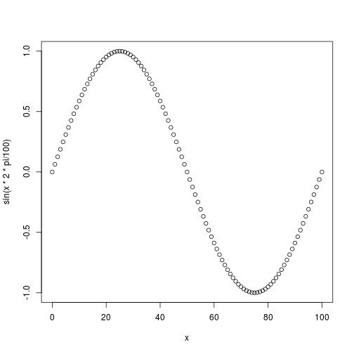
The environment is dynamic, but under your control!
- Variables do not persist between sessions (unless loaded from .Rdata 😢)
- Variables only change their value on re-assignment
Editor
The console is for evaluating commands you don’t intend to keep or reuse. It’s useful for testing commands and poking around. The environment represents the state of a current session. The editor reads and writes files–it is where you head to compose your R scripts.
R scripts are simple text files that contain code you intend to run again and
again; code to process data, perform analyses, produce visualizations, and even
generate reports. The editor and console work together in the RStudio IDE, which
gives you multiple ways to send parts of the script you are editing to the
console for immediate evaluation. Alternatively you can “source” the entire
script or run it from a shell with Rscript.
Open up “worksheet.R” in the editor, and follow along by
replacing the ... placeholders with the code here. Then evalute just this line
(Ctrl+Enter on Windows, ⌘+Enter on macOS)
vals <- seq(1, 100)
Our call to the function seq could have been much more explicit. We could give
the arguments by the names that seq is expecting.
vals <- seq(from = 1,
  to = 100)
Run that code by moving your cursor anywhere within those two lines and clicking “Run”, or by using the keyboard shortcut Ctrl-Return or ⌘ Return.
- Question
- What’s an advantage of naming arguments?
- Answer
- One advantage is that you can put them in any order. A related advantage is that you can then skip some arguments, which is fine to do if each skipped argument has a default value. A third advantage is code readability, which you should always be conscious of while writing in the editor.
Readability
Code readability in the editor cuts both ways: sometimes verbosity is useful, sometimes it is cumbersome.
The seq() function has an alternative form available when only the from and
to arguments are needed.
> 1:100
  [1]   1   2   3   4   5   6   7   8   9  10  11  12  13  14  15  16  17  18
 [19]  19  20  21  22  23  24  25  26  27  28  29  30  31  32  33  34  35  36
 [37]  37  38  39  40  41  42  43  44  45  46  47  48  49  50  51  52  53  54
 [55]  55  56  57  58  59  60  61  62  63  64  65  66  67  68  69  70  71  72
 [73]  73  74  75  76  77  78  79  80  81  82  83  84  85  86  87  88  89  90
 [91]  91  92  93  94  95  96  97  98  99 100
The : operator should be used whenever possible because it replaces a common,
cumbersome function call with an brief, intuitive syntax. Likewise, the assign
function duplicates the functionallity of the <- symbol, but is never used
when the simpler operator will suffice.
Function documentation
How would you get to know these properties and the names of a function’s arguments?
> ?seq
How would you even know what function to call?
> ??sequence
Load Data
We will use the function read.csv() to load data from a Comma Separated Value
(CSV) file. The essential argument for the function to read in data is the path to
the file, other optional arguments adjust how the file is read.
Additional file types can be read in using read.table(); in fact, read.csv()
is a simple wrapper for the read.table() function having set some default
values for some of the optional arguments (e.g. sep = ",").
Use the assignment operator “<-“ to read data into a variable for subsequent operations.
Type read.csv( into the editor and then press tab to see what arguments
this function takes. Hovering over each item in the list will show a description
of that argument from the help documentation about that function. Specify the
values to use for an argument using the syntax name = value.
storm <- read.csv('data/StormEvents.csv')
- Question
- How does
read.csvdetermine the field names? - Answer
- The
read.csvcommand assumes the first row in the file contains column names. Look at?read.csvto see the defaultheader = TRUEargument. What exactly that means is described down in the “Arguments” section.
Missing data, as interpreted by the read.csv function, is controlled by the
na.strings argument. Override the default value of 'NA' with a character
vector.
You often need to specify multiple strings to interpret as missing values, such
as na.strings = c("missing", "no data", "< 0.05 mg/L", "XX", "-9999").
storm <- read.csv(
  'data/StormEvents.csv',
  na.strings = c('NA', 'UNKNOWN'))
The data viewer, opened with the function View() or the spreadsheet icon in the
Environment, is useful despite not being a full spreadsheet application.
> View(storm)
After reading in the “StormEvents.csv” file, you can explore what types of data
are in each column with the str() function, short for “structure”.
> str(storm)
'data.frame':	100 obs. of  42 variables:
 $ BEGIN_YEARMONTH  : int  200604 200601 200601 200601 200601 200601 200601 200601 200601 200601 ...
 $ BEGIN_DAY        : int  7 1 1 1 1 30 30 28 28 28 ...
 $ BEGIN_TIME       : int  1515 0 0 0 0 500 500 800 1400 800 ...
 $ END_YEARMONTH    : int  200604 200601 200601 200601 200601 200601 200601 200601 200601 200601 ...
 $ END_DAY          : int  7 31 31 31 31 31 31 29 29 29 ...
 $ END_TIME         : int  1515 2359 2359 2359 2359 1400 1400 1300 500 1600 ...
 $ EPISODE_ID       : int  207534 202408 202409 202409 202409 202394 202394 202395 202396 202397 ...
 $ EVENT_ID         : int  5501658 5482479 5482480 5482481 5482482 5482324 5482325 5482326 5482327 5482328 ...
 $ STATE            : chr  "INDIANA" "COLORADO" "UTAH" "UTAH" ...
 $ STATE_FIPS       : int  18 8 49 49 49 8 8 8 8 8 ...
 $ YEAR             : int  2006 2006 2006 2006 2006 2006 2006 2006 2006 2006 ...
 $ MONTH_NAME       : chr  "April" "January" "January" "January" ...
 $ EVENT_TYPE       : chr  "Thunderstorm Wind" "Drought" "Drought" "Drought" ...
 $ CZ_TYPE          : chr  "C" "Z" "Z" "Z" ...
 $ CZ_FIPS          : int  51 12 23 29 24 4 13 13 5 4 ...
 $ CZ_NAME          : chr  "GIBSON" "WEST ELK AND SAWATCH MOUNTAINS" "EASTERN UINTA MOUNTAINS" "CANYONLANDS / NATURAL BRIDGES" ...
 $ WFO              : chr  "PAH" "GJT" "GJT" "GJT" ...
 $ BEGIN_DATE_TIME  : chr  "07-APR-06 15:15:00" "01-JAN-06 00:00:00" "01-JAN-06 00:00:00" "01-JAN-06 00:00:00" ...
 $ CZ_TIMEZONE      : chr  "CST" "MST" "MST" "MST" ...
 $ END_DATE_TIME    : chr  "07-APR-06 15:15:00" "31-JAN-06 23:59:00" "31-JAN-06 23:59:00" "31-JAN-06 23:59:00" ...
 $ INJURIES_DIRECT  : int  0 0 0 0 0 0 0 0 0 0 ...
 $ INJURIES_INDIRECT: int  0 0 0 0 0 0 0 0 0 0 ...
 $ DEATHS_DIRECT    : int  0 0 0 0 0 0 0 0 0 0 ...
 $ DEATHS_INDIRECT  : int  0 0 0 0 0 0 0 0 0 0 ...
 $ DAMAGE_PROPERTY  : chr  "60K" NA NA NA ...
 $ DAMAGE_CROPS     : chr  NA NA NA NA ...
 $ SOURCE           : chr  "GENERAL PUBLIC" "GOVT OFFICIAL" "GOVT OFFICIAL" "GOVT OFFICIAL" ...
 $ MAGNITUDE        : num  61 NA NA NA NA NA NA NA NA NA ...
 $ MAGNITUDE_TYPE   : chr  "EG" NA NA NA ...
 $ BEGIN_RANGE      : int  4 NA NA NA NA NA NA NA NA NA ...
 $ BEGIN_AZIMUTH    : chr  "E" NA NA NA ...
 $ BEGIN_LOCATION   : chr  "PATOKA" NA NA NA ...
 $ END_RANGE        : int  NA NA NA NA NA NA NA NA NA NA ...
 $ END_AZIMUTH      : chr  NA NA NA NA ...
 $ END_LOCATION     : chr  "OAKLAND CITY" NA NA NA ...
 $ BEGIN_LAT        : num  38.4 NA NA NA NA ...
 $ BEGIN_LON        : num  -87.5 NA NA NA NA ...
 $ END_LAT          : num  38.3 NA NA NA NA ...
 $ END_LON          : num  -87.3 NA NA NA NA ...
 $ EPISODE_NARRATIVE: chr  NA "The storm track favored northwest Colorado with respect to snowfall and increased snowpack. In contrast, cold s"| __truncated__ "The storm track favored northeast Utah with respect to snowfall and increased snowpack, while cold season preci"| __truncated__ "The storm track favored northeast Utah with respect to snowfall and increased snowpack, while cold season preci"| __truncated__ ...
 $ EVENT_NARRATIVE  : chr  "At Wheeling, the windows were blown out of a church, and holes were in some vinyl siding. Between Wheeling and "| __truncated__ NA NA NA ...
 $ DATA_SOURCE      : chr  "PDS" "PDS" "PDS" "PDS" ...
Data Structures
The str() function just showed us that our data is made up of one-dimensional data structures (columns).
There are two one-dimensional data structures you will regularly encounter.
- Lists
- Vectors
Lists
Lists are one-dimensional and each element is entirely unrestricted; you can put anything in a list.
Create a list called x with a string, a sequence, and a function.
x <- list('abc', 1:3, sin)
All data frames are actually lists, so our data frame storm is actually a list. We’ll get into more details later, but you can check this out with the function typeof().
> typeof(storm)
[1] "list"
- Question
- Compare the structure of
stormandxwhile thinking about the length of each of their elements. Do the elements within listxhave a length? The same length? - Answer
- The elements of
xall have lengths, and are not all the same. Note that the commandlength('abc')yields1.
When you enter a single number or character string in R, you are actually creating a one-dimensional data structure of length 1. There are not really 0-dimensional “scalars” in R. The kind of one-dimensional structure created in this is called a “vector”.
Vectors
Vectors are one-dimensional but unlike lists, values must be of the same data type (e.g. integer, character, logical).
Create a vector by combining elements of the same type together using the concatenate function c().
Type ?c() in the console to learn more about this really common and useful function.
> c(1, 2, 3)
[1] 1 2 3
All elements of a vector must be the same type, so when you attempt to combine different types they will be coerced to the most flexible type.
> c(1, 2, 'c')
[1] "1" "2" "c"
The difference between c(1, 2, 3) and c(1, 2, 'c') isn’t just in the third
element. To understand the difference, we need to recognize data types.
Data Types
Here is a summary of the data types you frequently encounter in R.
| Type | Example |
|---|---|
| double | 3.1, 4, Inf, NaN |
| integer | 4L, length(…) |
| character | ‘a’, ‘4’, ‘👏’ |
| logical | TRUE, FALSE |
| factor | “category1”, “category2” |
Both the double and integer data types are considered numeric, and while
the str function tells you that a double is “num”, the typeof function
will properly identify either numeric type.
Missing data created with NA actually have a variant for each data type. So you can put
NA in any vector without breaking the rule that the elements of a vector have the same
data type.
Factors
Data of type factor is stored in a vector that can only contain predefined values of
categorical data. Factors are similar to character vectors, but possess a levels
attribute that assigns names to each level, or distinct value, in the vector.
Use factor() to create a vector with predefined values, which are often
character strings.
education <- factor(
    c('college', 'highschool', 'college', 'middle', 'middle'),
    levels = c('middle', 'highschool', 'college'))
The str function identifies this vector as being of data type “factor” and notes the labels for each level, but prints the integers assigned to the levels instead of the labels.
> str(education)
Factor w/ 3 levels "middle","highschool",..: 3 2 3 1 1
Factors can sometimes be tricky to work with in R. While factors can be useful for plotting data by categories, they can often get in the way of other calculations and analyses. It is good to know how to convert between data types with the functions as.character(), as.integer(), as.factor(), as.numeric().
Data Frames
We mentioned above that a data frame is actually a list of vectors, but with a few important constraints. The vectors must all be of the same length, giving a rectangular data structure. Vectors must also each have a unique name (column name).
Use the dim() function to check the dimensions of our storm data frame.
> dim(storm)
[1] 100 42
The column names are accessed by the names() function.
> names(storm)
 [1] "BEGIN_YEARMONTH"   "BEGIN_DAY"         "BEGIN_TIME"
 [4] "END_YEARMONTH"     "END_DAY"           "END_TIME"
 [7] "EPISODE_ID"        "EVENT_ID"          "STATE"
[10] "STATE_FIPS"        "YEAR"              "MONTH_NAME"
[13] "EVENT_TYPE"        "CZ_TYPE"           "CZ_FIPS"
[16] "CZ_NAME"           "WFO"               "BEGIN_DATE_TIME"
[19] "CZ_TIMEZONE"       "END_DATE_TIME"     "INJURIES_DIRECT"
[22] "INJURIES_INDIRECT" "DEATHS_DIRECT"     "DEATHS_INDIRECT"
[25] "DAMAGE_PROPERTY"   "DAMAGE_CROPS"      "SOURCE"
[28] "MAGNITUDE"         "MAGNITUDE_TYPE"    "BEGIN_RANGE"
[31] "BEGIN_AZIMUTH"     "BEGIN_LOCATION"    "END_RANGE"
[34] "END_AZIMUTH"       "END_LOCATION"      "BEGIN_LAT"
[37] "BEGIN_LON"         "END_LAT"           "END_LON"
[40] "EPISODE_NARRATIVE" "EVENT_NARRATIVE"   "DATA_SOURCE"
Creating a data frame from scratch can be done by combining vectors with the
data.frame() function. We created the education vector above. Now create a
vector named income, and put the two vectors together to make a data frame.
income <- c(32000, 28000, 89000, 0, 0)
df <- data.frame(education, income)
In summary, a data frame is the data structure most similar to a spreadsheet, with a few key differences:
- The columns must be equal-length vectors.
- As vectors, a column must hold values of the same type.
- Each column must have a unique name.
Remember to use these functions when getting to know a data frame:
dim() |
dimensions |
nrow(), ncol() |
number of rows, columns |
names() |
(column) names |
str() |
structure |
summary() |
summary info |
head() |
shows first few rows |
tail() |
shows last few rows |
Matrices
The matrix is a two-dimensional data structure, and differs from a data frame in terms
of the underlying data type. A matrix must be composed of elements of the same data type. You can check to see if you have a matrix by using the class() function.
When should you use a matrix vs. a data frame?
If your columns of data have different data types (e.g. integer, character, factor), you need to use a data frame.
If the analysis or functions you are using expect one structure or the other, you should use the expected data structure
Data structure quick reference:
| Data Dimensions | Data Type: Homogeneous |
Data Type: Heterogeneous |
|---|---|---|
| 1-D | c() |
list() |
| 2-D | matrix() |
data.frame() |
| n-D | array() |
Parts and Subsets
Any single part of a data structure is always accessible, either by its name or
by its position, using double square brackets: [[ and ]].
Position
The first element:
> income[[1]]
[1] 32000
The third element:
> income[[3]]
[1] 89000
Names
Parts of an object may also have a name. The names can be given when you are
creating a vector or afterwards using the names() function.
> df[['education']]
[1] college    highschool college    middle     middle
Levels: middle highschool college
names(df) <- c('ed', 'inc')
> df[['ed']]
[1] college    highschool college    middle     middle
Levels: middle highschool college
- Question
- This use of
<-withnames(x)on the left is a little odd. What’s going on? - Answer
- We are overwriting an existing variable, but one that is accessed through the output of the function on the left rather than the global environment.
For a multi-dimensional array, separate the dimensions within which a part is requested with a comma.
> df[[3, 'ed']]
[1] college
Levels: middle highschool college
It’s fine to mix names and indices when selecting parts of an object.
The $ sign is an additional operator for quick access to a single, named part
of some objects. It’s most useful when used interactively with “tab completion” on
the columns of a data frame.
> df$ed
[1] college    highschool college    middle     middle
Levels: middle highschool college
Subsets
Multiple parts of a data structure are similarly accessed using single square
brackets: [ and ]. What goes between the brackets, to specify the positions
or names of the desired subset, may be of multiple forms.
| Parts | Result |
|---|---|
| positives | elements at given positions |
| negatives | given positions omitted |
| logicals | elements where the corresponding position is TRUE |
| nothing | all the elements |
days <- c(
  'Sunday', 'Monday', 'Tuesday',
  'Wednesday', 'Thursday', 'Friday',
  'Saturday')
weekdays <- days[2:6]
weekend <- days[c(1, 7)]
> weekdays
[1] "Monday" "Tuesday" "Wednesday" "Thursday" "Friday"
> weekend
[1] "Sunday" "Saturday"
A logical test applied to a single column produces a vector of TRUE and
FALSE values that’s the right length for subsetting the data.
> df[df$ed == 'college', ]
       ed    in
1 college 32000
3 college 89000
Functions
Functions package up a batch of commands. There are several reasons to develop functions in R for data analysis:
- reuse
- readability
- modularity
- consistency
If you find yourself copy-pasting code, or see blocks of similar code through your project, those are candidates for being moved into functions. Writing functions prevents you from duplicating code, making errors from copy-pasting that are difficult to troubleshoot, and is a real time-saver when you want to update what the function does. If you’re doing something more than twice, write a function!
Anatomy of a function
Like all programming languages, R has keywords that are reserved for important
activities, like creating functions. Keywords are usually very intuitive; the
one we need is function.
function(...) {
    ...
    return(...)
}
Three components of a function:
- arguments: control how you can call the function
- body: the code inside the function
- return value: controls what output the function gives
> function(arguments) {
+     body
+     return(return_value)
+ }
We’ll make a function to extract the first row of its argument, which we give the
placeholder name a to use inside the function:
function(a) {
    result <- a[1, ]
    return(result)
}
Note that a doesn’t exist outside our function. Our function contains
the instructions for how any a will be handled. We supply what a is as the
argument when we call the function.
Finally, we need to give the function a name so we can use it like we used c()
and seq() above.
first <- function(a) {
    result <- a[1, ]
    return(result)
}
Now we can call our function, and supply the argument df.
> first(df)
       ed    in
1 college 32000
- Question
- Can you explain the result of entering
first(income)into the console? - Answer
- The function caused an error, which prompted the interpreter to print a helpful error message. Never ignore an error message. (It’s okay to ignore a “warning”.)
Flow Control
A generic term for causing the interpreter to repeat or skip certain lines, using concepts like “for loops” and conditionals.
The R interpreter’s “focus” flows through a script (or any section of code you run) line by line. Without additional instruction, every line is processed from the top to bottom. Flow control refers mostly to the two main ways of directing the interpreter’s focus, via loops and conditions.
Flow control happens within blocks of code isolated between curly braces { and
}, known as “statements”.
if (...) {
    ...
} else {
    ...
}
The keyword if must be followed by a logical test which determines, at
runtime, what to do next. The R interpreter goes to the first statement if the
logical value is TRUE and to the second statement if it’s FALSE.
> if (logical_test) {
+     statement_1
+ } else {
+     statement_2
+ }
Let’s try building a simple if/else statement.
This tests whether the first element in the ed column of our data frame df contains the word “college”. If it does, it prints the first element of the inc column. Otherwise, it prints “no college education”.
if (df$ed[1] == "college") {
    print(df$inc[1])
} else {
    print("no college education")
}
An if/else conditional would allow the first() function we wrote previously to avoid the error
thrown by calling first(counts).
first <- function(dat) {
    if (is.vector(dat)) {
        result <- dat[[1]]
    } else {
        result <- dat[1, ]
    }
    return(result)
}
> first(df)
       ed   inc
1 college 32000
> first(income)
[1] 32000
Distributions and Statistics
Since it was designed by statisticians, R can easily draw random numbers from probability distributions and calculate probabilities.
To generate random numbers from a normal distribution, use the function
rnorm()
rnorm(n = 10)
 [1] -0.2370723 -1.4292213  0.8261260  1.6549967  0.7993259  1.0656807
 [7] -0.3397285 -0.2609470 -0.2047979 -0.1227364
| Function | Returns | Notes |
|---|---|---|
rnorm() |
Draw random numbers from normal distribution | Specify n, mean, sd |
dnorm() |
Probability density at a given number | |
pnorm() |
Cumulative probability up to a given number | left-tailed by default |
qnorm() |
The quantile given a cumulative probability | opposite of pnorm |
Statistical distributions and their functions. See Table 14.1 in R for Everyone by Jared Lander for a full table.
| Distribution | Functions |
|---|---|
| Normal | *norm |
| Binomial | *binom |
| Poisson | *pois |
| Gamma | *gamma |
| Exponential | *exp |
| Uniform | *unif |
| Logistic | *logis |
R has built in functions for handling many statistical tests.
x <- rnorm(n = 100, mean = 15, sd = 7)
y <- rbinom(n = 100, size = 20, prob = .85)
The samples above are drawn from different distributions with different means. The T-Test should easily distinguish them, although it does not check assumptions!
> t.test(x, y)
	Welch Two Sample t-test

data:  x and y
t = -3.0895, df = 107.92, p-value = 0.00255
alternative hypothesis: true difference in means is not equal to 0
95 percent confidence interval:
 -3.3562439 -0.7327582
sample estimates:
mean of x mean of y
  15.2155   17.2600
Shapiro’s test of normality provides one routine for verifying assumptions.
> shapiro.test(y)
	Shapiro-Wilk normality test

data:  y
W = 0.94755, p-value = 0.0005739
Review
In this introduction to R, we touched on several key parts of scripting for data analysis.
- RStudio panes
- variable assignment
- data structures
- subsetting data
- functions
- flow control
- probabilities
Special characters in R
Perhaps more than most languages, an R script can appear like a jumble of archaic symbols. Here is a little table of characters to recognize as having special meaning.
| Symbol | Meaning |
|---|---|
? |
get help |
# |
comment |
: |
sequence |
::, ::: |
access namespaces (advanced) |
<- |
assignment |
$, [ ], [[ ]] |
subsetting |
% % |
infix operators, e.g. %*% |
{ } |
statements |
. |
|
@ |
slot (advanced) |
The . in R has no fixed meaning and is often used as _ might be used to
separate words in a variable name.
Exercises
Exercise 1
Use the quadratic formula to find \(x\) that satisfies the equation \(1.5 x^2 + 0.3 x - 2.9 = 0\).
\[\frac{-0.3 \pm \sqrt{0.3^2 - 4 \times 1.5 \times {-2.9}}}{2 \times 1.5}\]Exercise 2
By default, all character data is read in to a data.frame as factors. Use the
read.csv() argument stringsAsFactors to suppress this behavior, then
subsequently modify the STATE column in storm to make it a factor. Remember
that columns of a data.frame are identified to the R interpreter with the $
operator, e.g. storm$STATE.
Exercise 3
Use the typeof function to inspect the data type of income, and do the same
for another variable to which you assign a list of numbers. Why are they
different? Use c to combine income with the new variable you just created
and inspect the result with typeof. Does c always create vectors?
Exercise 4
Create a data frame with two columns, one called “species” with four strings and
another called “abund” with four numbers. Store your data frame as a variable
called data.
Exercise 5
- Get weekdays using negative integers.
- Get M-W-F using a vector of postitions generated by
seq()that uses thebyargument (don’t forget to?seqfor help).
Exercise 6
The keywords else and if can be combined to allow flow control among more
than two statements, as below. Expand the first function once again to
differentiate between dat provided as a matrix and as a data.frame. It’s
up to you what the “first” element of a matrix should be!
if (...) {
  ...
} else if {
  ...
} else {
  ...
}
Solutions
Solution 1
(-0.3 + sqrt(0.3 ^ 2 - 4 * 1.5 * -2.9)) / (2 * 1.5)
[1] 1.294035
Solution 2
storm <- read.csv(
  'data/StormEvents.csv',
  stringsAsFactors = FALSE)
storm$STATE <- factor(storm$STATE)
Solution 3
x <- list(3, 4, 5, 7)
typeof(x)
[1] "list"
The variable x has a data type of list, so R does not restrict its elements
to a particular type as it does for vectors.
typeof(c(income, x))
[1] "list"
The result of combining a list and vector is a list, because the list is the more flexible data structure.
Solution 4
species <- c('ape', 'bat', 'cat', 'dog')
abund <- 1:4
data <- data.frame(species, abund)
Solution 5
days[c(-1, -7)]
[1] "Monday" "Tuesday" "Wednesday" "Thursday" "Friday"
days[seq(2, 7, 2)]
[1] "Monday" "Wednesday" "Friday"
Solution 6
first <- function(dat) {
    if (is.vector(dat)) {
        result <- dat[[1]]
    } else if (is.matrix(dat)) {
        result <- dat[[1, 1]]
    } else {
        result <- dat[1, ]
    }
    return(result)
}
m <- matrix(1:9, nrow = 3, ncol = 3)
first(m)
[1] 1
If you need to catch-up before a section of code will work, just squish it's 🍅 to copy code above it into your clipboard. Then paste into your interpreter's console, run, and you'll be ready to start in on that section. Code copied by both 🍅 and 📋 will also appear below, where you can edit first, and then copy, paste, and run again.
# Nothing here yet!