Interactive Web Applications with Shiny

Lesson 8 with Kelly Hondula

Lesson Goals
Shiny components
Accessing data
Input and Output Objects
Design and Layout
Reactivity
Share your app
Solutions

Lesson Goals

This lesson presents an introduction to creating interactive web applications using the R Shiny package. It covers:

The basic building blocks of a Shiny app
How to create interactive elements, including plots
How to customize and arrange elements on a page

Data

This lesson makes use of several publicly available datasets that have been customized for teaching purposes, including the Portal teaching database.

What is Shiny?

Shiny is a web application framework for R that allows you to create interactive web apps without requiring knowledge of HTML, CSS, or JavaScript. These web apps can be used for exploratory data analysis and visualization, to facilitate remote collaboration, share results, and much more. The example below, and many additional examples, will open in a new browser window (you may need to prevent your broswer from blocking pop-out windows in order to view the app).

The shiny package includes some built-in examples to demonstrate some of its basic features. When applications are running, they are displayed in a separate browser window or the RStudio Viewer pane.

library(shiny)
runExample('01_hello')

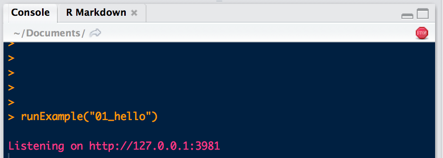
Notice back in RStudio that a stop sign appears in the Console window while your app is running. This is because the current R session is busy running your application.

Closing the app window may not stop the app from using your R session. Force the app to close when necessary by clicking the stop sign in the header of the Console window. The Console window prompt > should return.

Top of Section

Shiny components

Depending on the purpose and computing requirements of any Shiny app, you may set it up to run R code on your computer, a remote server, or in the cloud. However all Shiny apps consists of the same two main components:

The user interface (UI) which defines what users will see in the app and its design.
The server which defines the instructions for how to assemble components of the app like plots and input widgets.

Who or what is “Listening” on 127.0.0.1?

127.0.0.1 is the IP address your laptop uses for itself (it’s the same as ‘localhost’).
Your laptop is hosting a web page (the UI) whose content is controlled by a running R session.
When you run an app through RStudio, that R session is also running the server on your laptop.
The server responds when you interact with the web page, processing R commands and updating UI objects accordingly.

For big projects, the UI and server components may be defined in separate files called ui.R and server.R and saved in a folder representing the app.

my_app
├── ui.R
├── server.R
├── www
└── data

For ease of demonstration, we’ll use the alternative approach of defining UI and server objects in a R script representing the app.

# User Interface
ui <- ... 

# Server
server <- ...

# Create the Shiny App
shinyApp(ui = ui, server = server)

Hello, Shiny World!

Open worksheet-8-1.R in your handouts repository. In this file, define objects ui and server with the assignment operator <- and then pass them to the function shinyApp(). These are the basic components of a shiny app.

# User Interface
ui <- navbarPage(title = 'Hello, Shiny World!')

# Server
server <- function(input, output){}

# Create the Shiny App
shinyApp(ui = ui, server = server)

Notice the green Run App button appear when the file is saved. This button also allows you to control whether the app runs in a browser window, in the RStudio Viewer pane, or in an external RStudio window.

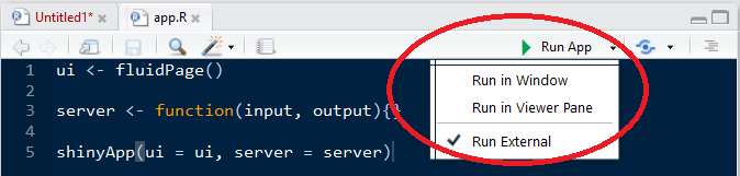
The shiny package must be installed for RStudio to identify files associated with a Shiny App and put up a green arrow with a Run App button. Note that the file names must be ui.R and server.R if these components are scripted in separate files.

Top of Section

Accessing data

Because the Shiny app is going to be using your local R session to run, it will be able to recognize anything that is loaded into your working environment.

Here, we read in CSV files from the Portal dataset, so it is available to both the ui and server definitions. The app script is in the same folder as data, and you only need to specify the relative file path.

# Data
species <- read.csv('data/species.csv', stringsAsFactors = FALSE)
animals <- read.csv('data/animals.csv', na.strings = '', stringsAsFactors = FALSE)

Shiny apps can also be designed to interact with remote data or shared databases.

Top of Section

Input and Output Objects

The user interface and the server interact with each other through input and output objects. The user’s interaction with input objects alters parameters in the server’s instructions – instructions for creating output objects shown in the UI.

Writing an app requires careful attention to how your input and output objects relate to each other, i.e. knowing what actions will initiate what sections of code to run at what time.

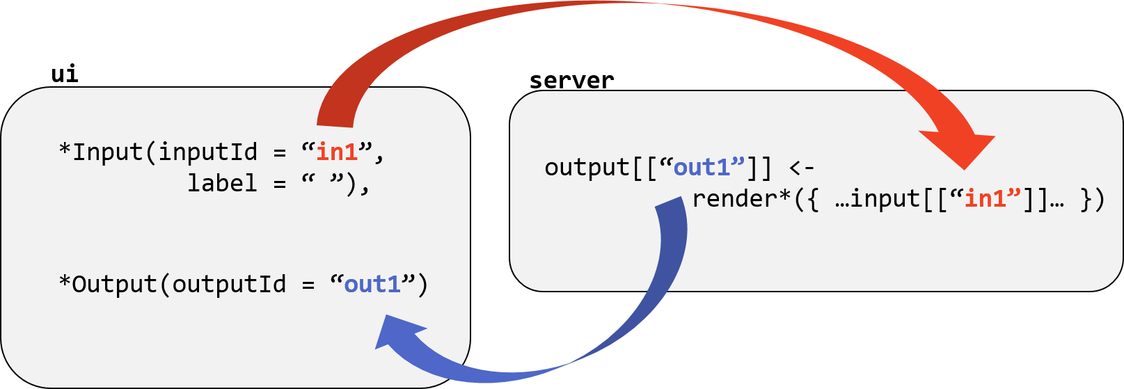
This diagrams input and output relationships within the UI and server objects:

Input objects are created and named in the UI with *Input() functions like selectInput() or radioButtons().
Data from input objects affects render functions in the server that create output objects.
Output objects are placed in the UI using *Output() functions like plotOutput() or textOutput().

Input Objects

Input objects collect information from the user and save it into a list. Input values can change when a user changes the input. These inputs can be many different things: single values, text, vectors, dates, or even files uploaded by the user.

The first two arguments for all input objects are:

inputId (notice the capitalization here!) which is for giving the input object a name to refer to in the server, and
label which is for text to display to the user.

See a gallery of input objects with sample code here

Define the UI by adding an input object that lets users select a species ID from the species table.

# User Interface
in1 <- selectInput(inputId = 'pick_species',
                   label = 'Pick a species',
                   choices = unique(species[['id']]))
...
tab <- tabPanel(title = 'Species', in1, ...)
ui <- navbarPage(title = 'Portal Project', tab)

Use the selectInput() function to create an input object called pick_species. Use the choices = argument to define a vector with the unique values in the species id column. Make the input object an argument to the function tabPanel(), preceded by a title argument. We will learn about design and layout in a subsequent section.

Other notes about input objects

Choices for inputs can be named using a list to match the display name to the value such as list('Male' = 'M', 'Female' = 'F').
Selectize inputs are a useful option for long drop down lists.
Always be aware of what the default value is for input objects you create.

Output objects

Output objects are created through the combination of a render*() function in the server and a paired *Output() functions in the UI.

Desired UI Object	`render*()`	`*Output()`
plot	renderPlot()	plotOutput()
text	renderPrint()	verbatimTextOutput()
text	renderText()	textOutput()
static table	renderTable()	tableOutput()
interactive table	renderDataTable()	dataTableOutput()

The server function adds the result of each render*() function to a list of output objects.

Textual Output

Render the species ID as text using renderText() in the server function, identifying the output as species_id.

# Server
server <- function(input, output) {
  output[['species_id']] <- renderText(input[['pick_species']])
}

Display the species ID as text in the user interface’s tabPanel as a textOutput object.

# User Interface
in1 <- selectInput(inputId = 'pick_species',
                   label = 'Pick a species',
                   choices = unique(species[['id']]))
out1 <- textOutput('species_id')
tab <- tabPanel(title = 'Species', in1, out1)
ui <- navbarPage(title = 'Portal Project', tab)

Here is the complete worksheet-8-2.R. Go ahead and run the app!

# Data
species <- read.csv('data/species.csv', stringsAsFactors = FALSE)
animals <- read.csv('data/animals.csv', na.strings = '', stringsAsFactors = FALSE)

# User Interface
in1 <- selectInput(inputId = 'pick_species',
                   label = 'Pick a species',
		   choices = unique(species[['id']]))
out1 <- textOutput('species_id')
tab <- tabPanel(title = 'Species', in1, out1)
ui <- navbarPage(title = 'Portal Project', tab)

# Server
server <- function(input, output) {
  output[['species_id']] <- renderText(input[['pick_species']])
  }

Render functions tell Shiny how to build an output object to display in the user interface. Output objects can be data frames, plots, images, text, or most anything you can create with R code to be visualized.

Use outputId names in quotes to refer to output objects within *Output() functions. Other arguments to *Output() functions can control their size in the UI as well as add advanced interactivity such as selecting observations to view data by clicking on a plot.

Note that it is also possible to render reactive input objects using the renderUI() and uiOutput() functions for situations where you want the type or parameters of an input object to change based on another input. For an exmaple, see “Creating controls on the fly” here.

Graphical Output

In worksheet-8-3.R, we use the animals table to plot abundance of the selected species, rather than just printing its id.

First, the server must filter the survey data based on the selected species, and then create a bar plot within the renderPlot() function. Don’t forget to import the necessary libraries.

# Server
server <- function(input, output) {
  output[['species_id']] <- renderText(input[['pick_species']])
  output[['species_plot']] <- renderPlot(
    animals %>%
      filter(species_id == input[['pick_species']]) %>%
      ggplot(aes(year)) +
        geom_bar()
  )
}

Second, use the corresponding plotOutput() function in the UI to display the plot in the app.

# User Interface
in1 <- selectInput(inputId = 'pick_species',
                   label = 'Pick a species',
                   choices = unique(species[['id']]))
out1 <- textOutput('species_id')
out2 <- plotOutput('species_plot')
tab <- tabPanel('Species', in1, out1, out2)
ui <- navbarPage(title = 'Portal Project', tab)

Exercise 1

Change out1 to have an outputId of “species_name” and modify the renderText() function to print the genus and species above the plot, rather than the species ID. Hint: The function paste() with argument collapse = ' ' will convert a data frame row to a text string.

View solution

Top of Section

Design and Layout

A suite of *Layout() functions make for a nicer user interface. You can organize elements using pre-defined high level layouts such as

sidebarLayout()
splitLayout()
verticalLayout()

The more general fluidRow() allows any organization of elements within a grid. The folowing UI elements, and more, can be layered on top of each other in either a fluid page or pre-defined layouts.

tabsetPanel()
navlistPanel()
navbarPage()

Here is a schematic of nested UI elements inside the sidebarLayout(). Red boxes represent input objects and blue boxes represent output objects.

Each object is located within one or more nested panels, which are nested within a layout. Objects and panels that are at the same level of hierarchy need to be separated by commas in calls to parent functions. Mistakes in usage of commas and parentheses between UI elements is one of the first things to look for when debugging a shiny app!

To re-organize the elements of the “Species” tab using a sidebar layout, we modify the UI to specify the sidebar and main elements.

# User Interface
in1 <- selectInput('pick_species',
                   label = 'Pick a species',
                   choices = unique(species[['id']]))
out1 <- plotOutput('species_name')
out2 <- plotOutput('species_plot')
side <- sidebarPanel('Options', in1)
main <- mainPanel(out1, out2)
tab <- tabPanel('Species',
                sidebarLayout(side, main))
ui <- navbarPage(title = 'Portal Project', tab)

Exercise 2

Include a tabset within the main panel. Call the first element of the tabset “Plot” and show the current plot. Call the second element of the tabset “Data” and show an interactive table with the animals data used in the plot.

View solution

Notice the many features of the data table output. There are many options that can be controlled within the render function such as pagination and default length. See here for examples and how to extend this functionality using JavaScript.

General layouts

The fluidPage() layout design consists of rows which contain columns of elements. To use it, first define the width of an element relative to a 12-unit grid within each column using the function fluidRow() and listing columns in units of 12. The argument offset can be used to add extra spacing. For example:

fluidPage(
  fluidRow(
    column(4, '4'),
    column(4, offset = 4, '4 offset 4')      
  ),
  fluidRow(
    column(3, offset = 3, '3 offset 3'),
    column(3, offset = 3, '3 offset 3')  
  ))

Customization

Along with input and output objects, you can add headers, text, images, links, and other html objects to the user interface using “builder” functions. There are shiny function equivalents for many common html tags such as h1() through h6() for headers. You can use the console to see that the return from these functions produce HTML code.

h5('This is a level 5 header')

<h5>This is a level 5 header</h5>

a(href = 'www.sesync.org', 'This syntax renders a link')

<a href="www.sesync.org">This syntax renders a link</a>

Exercise 3

Use the img builder function to add a logo, photo, or other image to your app. The help under ?img states that HTML attributes come from named arguments to img, and the “img” HTML tag requires two. You’ll need to save the image file in a subfolder called “www”.

View solution

Some useful features and resources

In addition to titles for tabs, you can also use icons.
Use the argument position = 'right' in the sidebarLayout() function if you prefer to have the side panel appear on the right.
See here for additional html tags you can use.
For large blocks of text consider saving the text in a separate markdown, html, or text file and use an include* function (example).
Add images by saving those files in a folder called www. Embed it with img(src='%filename%')
Use a shiny theme with the shinythemes package

Top of Section

Reactivity

Input objects are reactive which means that an update to this value by a user will notify objects in the server that its value has been changed.

The outputs of render functions are called observers because they observe all “upstream” reactive values for changes.

Reactive objects

The code inside the body of render*() functions will re-run whenever a reactive value (e.g. an input objet) inside the code is changed by the user. When any observer is re-rendered, the UI is notified that it has to update.

Question: Which element is an observer in the app within worksheet-8-3.R.
Answer: The object created by renderPlot() and stored with outputId “species_plot”.

In worksheet-8-4.R we’re going to create a new input object in the sidebar panel that constrains the plotted data to a user defined range of months.

in2 <- sliderInput('slider_months',
                   label = 'Month Range',
                   min = 1,
                   max = 12,
                   value = c(1, 12))
side <- sidebarPanel('Options', in1, in2)

To limit animals to the user specified months, an additional filter is needed within the renderPlot() function like

filter(month %in% ...)

In order for filter() to dynamically respond to the slider, whatever replaces ... must react to the slider.

Shiny provides the reactive() function for such times when an appropriate *Input() object isn’t available. The value returned by reactive() will also be a function.

filter(month %in% reactive_seq())

The %in% test within filter() needs a sequence, so we wrap seq in reactive to generate a function that takes no direct input.

reactive_seq <- reactive(
    seq(input[['slider_months']][1],
        input[['slider_months']][2])
    )

The reactive_seq can now be embedded in the renderPlot() and renderDataTable() functions.

# Server
server <- function(input, output) {

    reactive_seq <- reactive(
        seq(input[['slider_months']][1],
            input[['slider_months']][2])
    )
    output[['species_plot']] <- renderPlot(
        animals %>%
            filter(species_id == input[['pick_species']]) %>%
            filter(month %in% reactive_seq()) %>%
        ggplot(aes(year)) +
            geom_bar()
    )
    output[['species_table']] <- renderDataTable(
        animals %>%
            filter(species_id == input[['pick_species']]) %>%
            filter(month %in% reqctive_seq())
    )
}

Exercise 4

Notice the exact same code exists twice within the server function, once for renderPlot() and once for renderDataTable. Replace reactive_seq with a new reactive_data_frame that returns the filtered data.frame. Bask in the knowledge of how much CPU time you’ll save.

Top of Section

Once you have made an app, there are several ways to share it with others. It is important to make sure that everything the app needs to run (data and packages) will be loaded into the R session.

There is a series of articles on the RStudio website here about deploying apps.

share the source code in app.R (or ui.R and server.R) along with all required data files
if sharing through a GitHub repository, advertise that your app can be cloned and run with shiny::runGitHub('%repo%', '%username%')

To share just the UI (i.e. the web page), your app will need to be hosted by a server able to run the R code that powers the app while also acting as a public web server. There is limited free hosting available through RStudio with shinapps.io. SESYNC maintains a Shiny Apps server for our working group participants, and many other research centers are doing the same.

Top of Section

Solutions

Solution 1

# Libraries
library(ggplot2)
library(dplyr)

# Data
species <- read.csv('data/species.csv', stringsAsFactors = FALSE)
animals <- read.csv('data/animals.csv', na.strings = '', stringsAsFactors = FALSE)

# User Interface
in1 <- selectInput('pick_species',
                   label = 'Pick a species',
                   choices = unique(species[['id']]))
out1 <- textOutput('species_name')
out2 <- plotOutput('species_plot')
tab <- tabPanel(title = 'Species',
                in1, out1, out2)
ui <- navbarPage(title = 'Portal Project', tab)

server <- function(input, output) {
  output[['species_name']] <- renderText(
    species %>%
      filter(id == input[['pick_species']]) %>%
      select(genus, species) %>%
      paste(collapse = ' ')
  )
  output[['species_plot']] <- renderPlot(
    animals %>%
      filter(species_id == input[['pick_species']]) %>%
      ggplot(aes(year)) +
      geom_bar()
  )
}

# Create the Shiny App
shinyApp(ui = ui, server = server)

Return

Solution 2

# Libraries
library(ggplot2)
library(dplyr)

# Data
species <- read.csv('data/species.csv', stringsAsFactors = FALSE)
animals <- read.csv('data/animals.csv', na.strings = '', stringsAsFactors = FALSE)

# User Interface
in1 <- selectInput('pick_species',
                   label = 'Pick a species',
                   choices = unique(species[['id']]))
side <- sidebarPanel('Options', in1)
out1 <- textOutput('species_name')
out2 <- tabPanel(title = 'Plot',
                 plotOutput('species_plot'))
out3 <- tabPanel(title = 'Data',
                 dataTableOutput('species_table'))                 
main <- mainPanel(out1,
                  tabsetPanel(out2, out3))
tab <- tabPanel(title = 'Species',
                sidebarLayout(side, main))
ui <- navbarPage(title = 'Portal Project', tab)

server <- function(input, output) {
  output[['species_name']] <- renderText(
    species %>%
      filter(id == input[['pick_species']]) %>%
      select(genus, species) %>%
      paste(collapse = ' ')
  )
  output[['species_plot']] <- renderPlot(
    animals %>%
      filter(species_id == input[['pick_species']]) %>%
      ggplot(aes(year)) +
      geom_bar()
  )
  output[['species_table']] <- renderDataTable(
    animals %>%
      filter(species_id == input[['pick_species']])
  )
}

# Create the Shiny App
shinyApp(ui = ui, server = server)

Return

Solution 3

# Libraries
library(ggplot2)
library(dplyr)

# Data
species <- read.csv('data/species.csv', stringsAsFactors = FALSE)
animals <- read.csv('data/animals.csv', na.strings = '', stringsAsFactors = FALSE)

# User Interface
in1 <- selectInput('pick_species',
                   label = 'Pick a species',
                   choices = unique(species[['id']]))
img <- img(src = 'image-filename.png', alt = 'short image description')                   
side <- sidebarPanel(img, 'Options', in1)
out1 <- textOutput('species_name')
out2 <- tabPanel('Plot',
                 plotOutput('species_plot'))
out3 <- tabPanel('Data',
                 dataTableOutput('species_table'))                 
main <- mainPanel(out1,
                  tabsetPanel(out2, out3))
tab <- tabPanel(title = 'Species',
                sidebarLayout(side, main))
ui <- navbarPage(title = 'Portal Project', tab)

server <- function(input, output) {
  output[['species_name']] <- renderText(
    species %>%
      filter(id == input[['pick_species']]) %>%
      select(genus, species) %>%
      paste(collapse = ' ')
  )
  output[['species_plot']] <- renderPlot(
    animals %>%
      filter(species_id == input[['pick_species']]) %>%
      ggplot(aes(year)) +
      geom_bar()
  )
  output[['species_table']] <- renderDataTable(
    animals %>%
      filter(species_id == input[['pick_species']])
  )
}

# Create the Shiny App
shinyApp(ui = ui, server = server)

Return

Solution 4

# Libraries
library(ggplot2)
library(dplyr)

# Data
species <- read.csv('data/species.csv', stringsAsFactors = FALSE)
animals <- read.csv('data/animals.csv', na.strings = '', stringsAsFactors = FALSE)

# User Interface
in1 <- selectInput('pick_species',
                   label = 'Pick a species',
                   choices = unique(species[['id']]))
img <- img(src = 'image-filename.png', alt = 'short image description')
in2 <- sliderInput('slider_months',
                   label = 'Month Range',
                   min = 1,
                   max = 12,
                   value = c(1, 12))
side <- sidebarPanel(img, 'Options', in1, in2)									    
out1 <- textOutput('species_name')
out2 <- tabPanel('Plot',
                 plotOutput('species_plot'))
out3 <- tabPanel('Data',
                 dataTableOutput('species_table'))                 
main <- mainPanel(out1,
                  tabsetPanel(out2, out3))
tab <- tabPanel(title = 'Species',
                sidebarLayout(side, main))
ui <- navbarPage(title = 'Portal Project', tab)

# Server
server <- function(input, output) {
  reactive_data_frame <- reactive({
    months <- seq(input[['slider_months']][1],
                  input[['slider_months']][2])
    animals %>%
      filter(species_id == input[['pick_species']]) %>%
      filter(month %in% months)
  })
  output[['species_name']] <- renderText(
    species %>%
      filter(id == input[['pick_species']]) %>%
      select(genus, species) %>%
      paste(collapse = ' ')
  )
  output[['species_plot']] <- renderPlot(
    ggplot(reactive_data_frame(), aes(year)) +
      geom_bar()
  )
  output[['species_table']] <- renderDataTable(reactive_data_frame())
}

# Create the Shiny App
shinyApp(ui = ui, server = server)

Return

Top of Section

Interactive Web Applications with Shiny

Contents

Lesson Goals

Data

What is Shiny?

Shiny components

Who or what is “Listening” on 127.0.0.1?

Hello, Shiny World!

Accessing data

Input and Output Objects

Input Objects

Output objects

Textual Output

Graphical Output

Exercise 1

Design and Layout

Exercise 2

General layouts

Customization

Exercise 3

Some useful features and resources

Reactivity

Reactive objects

Exercise 4

Share your app

Share as files

Share as a website

Solutions

Solution 1

Solution 2

Solution 3

Solution 4