
May 31, 2021 by Quentin Read
These days, it seems like every time you turn around a new R package for making maps comes out, which renders an older one obsolete … it’s hard to keep track of! There are tons of competing alternatives for both traditional (static) maps and interactive maps. Tools like leaflet and mapview are great for interactive maps, but this post focuses on a classic: a static map. That’s right, no zooming in and out or panning back and forth. Just a nice clean simple map.

Static maps have been around for a long time — if it ain’t broke, don’t fix it.
This blog post was inspired by a request from a graduate student researcher in a SESYNC pursuit group who wanted to make a map displaying some raster data over a background of satellite imagery. In the past, she had used the ggmap package to put Google Earth imagery on her maps. That used to be free but recently Google started to charge money to access their imagery tiles through an API (though it is fairly cheap for light use). So she was looking for a free alternative. I did a lot of Googling and found lots of cool new stuff, including the ggspatial package, which makes an appearance later in this post (scroll to the bottom of this post for a list of packages to check out). I also found quite a few free or “freemium” tile servers that let you download satellite imagery tiles from an API to use in static or interactive maps. The one I liked the best was Mapbox, but I couldn’t find any R package to automate the process of downloading Mapbox tiles and adding them as background imagery for a map. So I wrote a little package of my own to do just that!
In this post I go through how to do the following, all from within R:
I wrote a very minimalist R package called qdrmapbox to package up all the code for this blog post in one place. It basically only does one thing, but it does that thing reasonably well (I think).
You can follow along with the code in the post or download an R script with all the code in one place.
First, install the package from the GitHub repo. The qdrmapbox package has a few other package dependencies that should install with it by default.
remotes::install_github('qdread/qdrmapbox')
Next you will have to sign up for a Mapbox account. Once you have one, create an API access token to access the Raster Tiles API. Save the token in a text file, containing only the token and nothing else. Using the token is free up to 750,000 tile requests, which is way more than enough for personal use, especially for creating interactive maps. Even if you built an interactive map, such as a Shiny app, it would take a good while to reach that limit.
These are the options I selected when I created the access token I used for this post.
Load the package!
library(qdrmapbox)
Now assign the API token to an invisible environment variable (obviously substitute ~/Documents/mapboxapikey.txt for the path and file name you used).
That is a good security practice — you don’t have to have the secret token in your script or workspace.
set_mapbox_api_key('~/Documents/mapboxapikey.txt')
In this example, we’re going to make a map of Maryland. Here are the lat-long coordinates of the northwest (upper left) and southeast (lower right) corners of the bounding box around Maryland.
zoom <- 8
upper_left <- c(39.8, -79.5)
lower_right <- c(37.8, -74.8)

md_tile_index <- find_tile_numbers(zoom = zoom, upper_left = upper_left, lower_right = lower_right)
Mapbox uses the OpenStreetMap tile numbering system.
Zoom level 8 means 2^8 by 2^8, or 256 by 256, tiles to cover the entire globe (this is the same numbering system used for the zoom levels of Google Maps, OpenStreetMap,
and other tile servers, so this tile index function will work for other things besides Mapbox). The output of find_tile_numbers() gives you the x and y indexes of the tiles.
At zoom level 8, we will need to download eight tiles (512 by 512 pixels apiece if we choose high resolution) to cover the state of Maryland.
You could always set the zoom level higher if you want higher resolution for a very large image.
md_tile_index

##   zoom  x  y
## 1    8 71 97
## 2    8 72 97
## 3    8 73 97
## 4    8 74 97
## 5    8 71 98
## 6    8 72 98
## 7    8 73 98
## 8    8 74 98
Now we’ll use the function download_mapbox_tiles() to request the tiles from the API, download them, and save the JPEG files to a local folder
(change the folder name and location in the code if you want). If the folder does not exist it will be created.
download_dir <- '~/mdtiles'

md_tile_df <- download_mapbox_tiles(tile_numbers_mat = md_tile_index, download_dir = download_dir, resolution = 'high', jpg_quality = 90)
The function download_mapbox_tiles() downloads the tiles into a local directory given the index numbers we just found.
Mapbox has low and high resolutions and JPEG quality settings of 70%, 80%, and 90%. I chose the highest in both cases.
We saved the output of download_mapbox_tiles() to a data frame called md_tile_df because it contains the file names of the
downloaded tiles which we can use in the next step to georeference.
head(md_tile_df, 2)

##   zoom  x  y                                                                  api_call                file_name         output_file_name
## 1    8 71 97 https://api.mapbox.com/v4/mapbox.satellite/8/71/97@2x.jpg90?access_token= ~/mdtiles/tile_71_97.jpg ~/mdtiles/tile_71_97.tif
## 2    8 72 97 https://api.mapbox.com/v4/mapbox.satellite/8/72/97@2x.jpg90?access_token= ~/mdtiles/tile_72_97.jpg ~/mdtiles/tile_72_97.tif
You can also see above how the API call is constructed. The base URL https://api.mapbox.com/v4/mapbox.satellite/ is followed by the zoom level,
tile x and y coordinates, the optional argument @2x for high resolution, and .jpg90 for 90% quality JPEG. Notice that the access token is not
included in the data frame. The API key is never included in any variable in the workspace. It’s only added to the API call when it’s actually used. Now that’s good security!

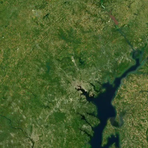
This is the Mapbox Satellite imagery tile containing SESYNC’s location at zoom level 8.
Okay, now we have a bunch of JPEGs, but they are not georeferenced, so we cannot use them to make a map yet. I was able to use information from this blog post by Jimmy Utterström and this post on GIS StackExchange to figure out how to do it.
The function georeference_all_tiles() uses GDAL to georeference the tiles, meaning to associate the images with geographical locations.
GDAL is a powerful system library for working with vector and raster geospatial data. Inside this function I call the command gdal_translate
to turn the JPEGs into GeoTIFF files by telling GDAL the coordinates of the corners of each tile.
Next we use build_virtual_raster(), which also uses GDAL under the hood, to mosaic the image tiles together into one “virtual raster,” or VRT file.
This function internally calls the command gdalbuildvrt and creates a VRT file called mdimage.vrt in the same directory as the .tif files.
The VRT file is a small text file that acts like a raster, though it’s only a pointer to the GeoTIFF tiles, so don’t delete the .tif files
once the .vrt file is created.
georeference_all_tiles(md_tile_df)

build_virtual_raster(md_tile_df, file.path(download_dir, 'mdimage.vrt'))
Now we have satellite imagery from Mapbox completely covering the state of Maryland, with a high enough resolution that we can use it for a good-quality map!
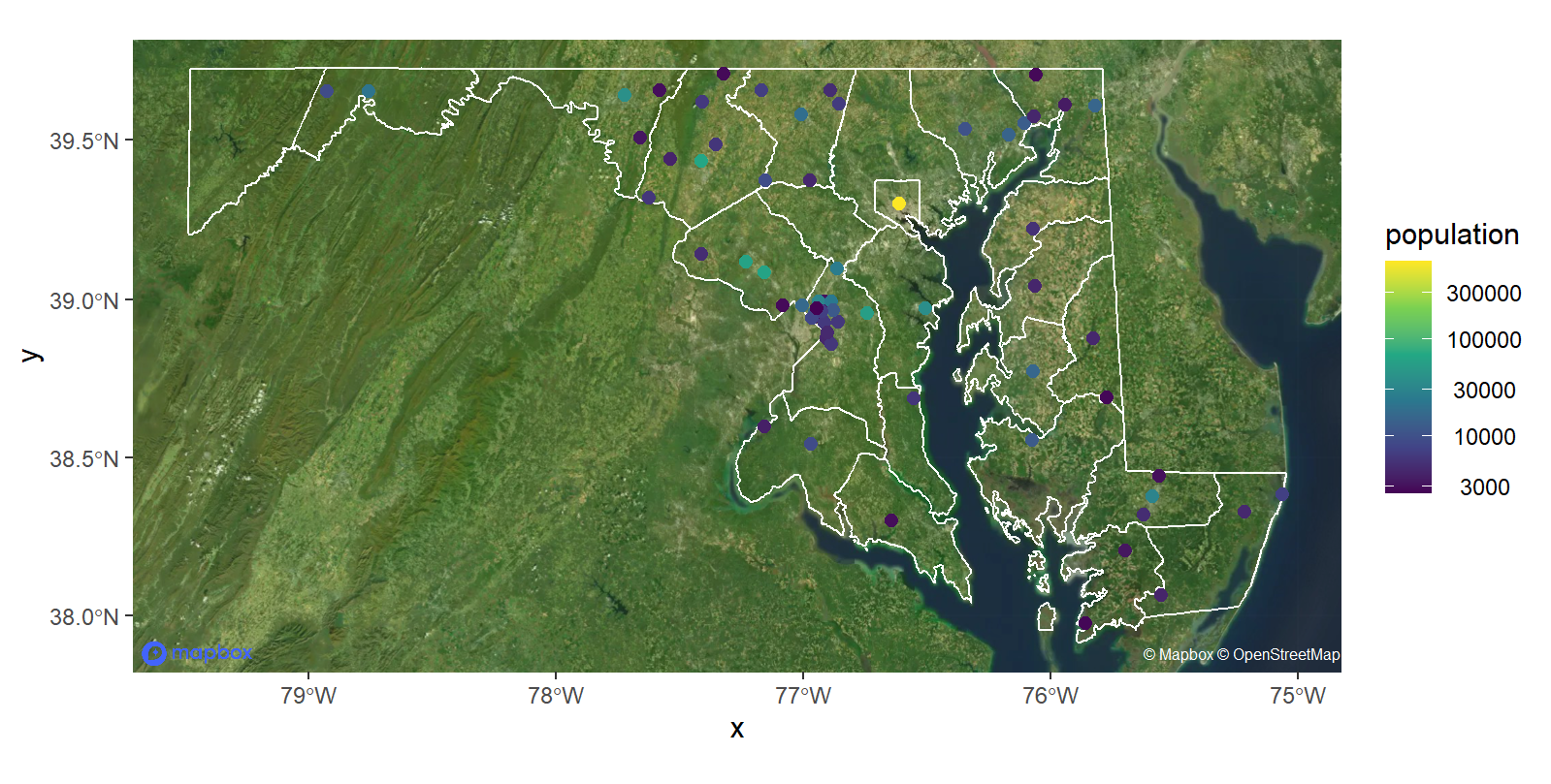
This is just a silly example using county boundary and city location data from the USAboundaries R package to plot the counties of Maryland and cities
colored by their population size on a log scale, with the satellite imagery from Mapbox as a background. The map is made with ggplot.
We use the function annotation_spatial() from the excellent ggspatial package to turn the raster to an “annotation” …
so it can be plotted in its true red-blue-green colors but doesn’t affect the fill or color scales of any of the actual data we plot on the map.
Load the packages we will need to make the map.
library(sf)
library(raster)
library(USAboundaries)
library(ggspatial)
library(ggplot2)
Now read in the satellite imagery as a raster stack (it’s a stack because it actually has three layers: the red, green, and blue).
mdimage_raster <- stack(file.path(download_dir, 'mdimage.vrt'))
Get some data to plot on the map: the county boundaries and city point locations for the state of Maryland.
md_counties <- us_counties(resolution = 'high', states = 'MD')
md_cities <- us_cities(states = 'MD')
Now make the map, with a little customization! I set alpha = 0.9 for the background image to make it slightly transparent because the image is a bit dark.
ggplot() +
  annotation_spatial(data = mdimage_raster, alpha = 0.9) +
  geom_sf(data = st_geometry(md_counties), color = 'white', fill = NA) +
  geom_sf(data = md_cities, aes(color = population), size = 2) +
  coord_sf(crs = 3857) +
  mapbox_logo(xmin = -8870000, xmax = -8820000, ymin = 4535000, ymax = 4590000) +
  annotate('text', x = Inf, y = -Inf, label = '\u00a9 Mapbox \u00a9 OpenStreetMap', hjust = 1, vjust = -1, color = 'white', size = 2) +
  scale_color_viridis_c(trans = 'log10', labels = function(x) format(x, scientific = FALSE))
Ta-da!

Final note: You have to be sure to give Mapbox proper credit following their attribution guidelines. When you use many of Mapbox’s services, the logo appears automatically in the corner.
But since we pulled these tiles manually, that doesn’t happen. So I wrote the function mapbox_logo() to put the mapbox logo on the map.
I supplied the coordinates in the “web Mercator” projection I used to display the map. Plus I also included the copyrights in the bottom right corner, all following the guidelines.
Here is a list of R packages that allow you to put open-source tile imagery onto static or interactive maps, and some additional resources for further reading. Disclaimer: I haven’t tried all of them out myself.