Documenting and Publishing your Data
Note: This lesson is in beta status! It may have issues that have not been addressed.
Handouts for this lesson need to be saved on your computer. Download and unzip this material into the directory (a.k.a. folder) where you plan to work.
Lesson Objectives
- Review key concepts of making your data tidy
- Discover the importance of metadata
- Learn what a data package is
- Prepare to publish your data from R
Specific Achievements
- Create metadata locally
- Build data package locally
- Learn how data versioning can help you collaborate more efficiently
- Practice uploading data package to repository (exercise outside lesson)
What is a data package?
A data package is a collection of files that describe your data.
There are two essential parts to a data package: data and metadata.
Data packages also frequently include code scripts that clean, process, or perform statistical anslyses on your data, and visualizations that are direct products of coded analyses. The relationships between these files are described in the provenance information for a data package. We will get into more details on these components in this lesson.
Why package and publish your data?
-
Data is a valuable asset - easily publish your data now or in the future
-
Efficient collaboration - improve sharing data with collaborators now
-
Credit for your work
-
Funder requirement
-
Publisher requirement
-
Open, Reproducible Science
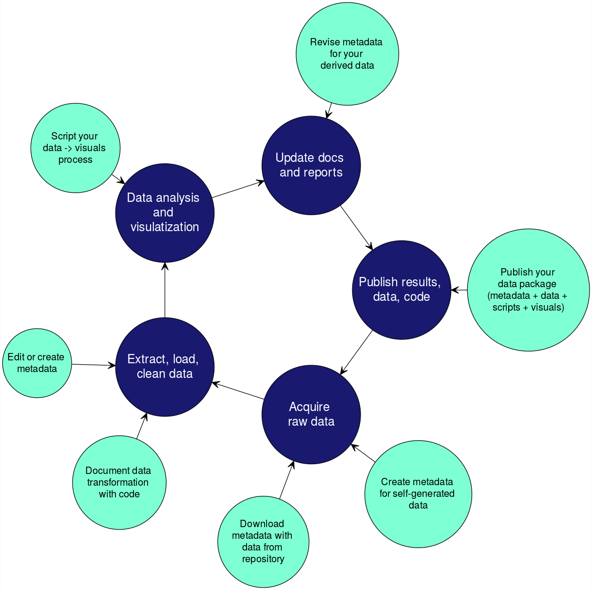
Integrating data documentation
It is important to incorporate documentation of your data throughout your reproducible research pipeline.
Preparing Data for Publication
Both raw data and derived data (data you’ve assembled or processed in some way) from a project need to be neat and tidy before publication. Following principles of tidy data from the beginning will make your workflows more efficient during a project, and will make it easier for others to understand and use your data once published. However, if your data isn’t yet tidy, you can make it tidier before you publish it.
Consistency is key when managing your data!
-
At a minimum, use the same terms to refer to the same things throughout your data.
- “origin”, not “starting place”, “beginning location”, and “source”
- “Orcinus orca”, not “killer Whale”, “Killer whale”, “killer.whale”, and “orca”
-
Consider using a discipline-wide published vocabulary if appropriate (ex: hydrological controlled vocab.)
Naming data files
Bad: “CeNsus data*2ndTry 2/15/2017.csv”
Good: “census_data.csv”
library(tidyverse)

stm_dat <- read_csv("data/StormEvents.csv")
Formatting data
- One table/file for each type of observation, e.g., a CSV file for storm events in the USA
- Each variable has its own column, e.g., month and location of a storm event are different columns in the file
- Each observation has its own row, e.g., each storm event is represented by a row
- Each value has its own cell
Downstream operations/analysis require tidy data.
These principles closely map to best practices for “normalization” in database design. R developer Hadley Wickham further describes the priciples of tidy data in this paper (Wickham 2014).
You can work towards ready-to-analyze data incrementally, documenting the intermediate data and cleaning steps you took in your scripts. This can be a powerful accelerator for your analysis both now and in the future.
Let’s do a few checks to see if our data is tidy.
- make sure data meet criteria above
- make sure blanks are NA or some other standard
> head(stm_dat)
> tail(stm_dat)
- check date format
> str(stm_dat)
- check case, white space, etc.
> unique(stm_dat$EVENT_NARRATIVE)
Outputting derived data
Because we followed the principle of one table/file for each type of observation, we have one table to be written out to a file now.
write_csv(stm_dat, "~/StormEvents_d2006.csv")
Versioning your derived data
Issue: Making sure you and your collaborators are using the same version of a dataset
One solution: version your data in a repository (more on this later)
What is Metadata?
Metadata is the information needed for someone else to understand and use your data. It is the Who, What, When, Where, Why, and How about your data.
This includes package-level and file-level metadata.
Common components of metadata
Package-level:
- Data creator
- Geographic and temporal extents of data (generally)
- Funding source
- Licensing information (Creative Commons, etc.)
- Publication date
File-level:
- Define variable names
- Describe variables (units, etc.)
- Define allowed values for a variable
- Describe file formats
Metadata Standards
The goal is to have a machine and human readable description of your data.
Metadata standards create a structural expression of metadata necessary to document a data set.
This can mean using a controlled set of descriptors for your data specified by the standard.
Without metadata standards, your digital data may be irretrievable, unidentifiable or unusable. Metadata standards contain definitions of the data elements and standardized ways of representing them in digital formats such as databases and XML (eXtensible Markup Language).
These standards ensure consistent structure that facilitates data sharing and searching, record provenance and technical processes, and manage access permissions. Recording metadata in digital formats such as XML ensures effective machine searches through consistent structured data entry, and thesauri using controlled vocabularies.
Metadata standards are often developed by user communities.
For example, the Ecological Metadata Language, EML, is a standard developed by ecologists to document environmental and ecological data. EML is a set of XML schema documents that allow for the structural expression of metadata. To learn more about EML check out their site.
Therefore, the standards can vary between disciplines and types of data.

Some examples include:
- General: Dublin Core
- Ecological/Environmental/Biological: EML, Darwin Core
- Social science: DDI, EAD
- Geospatial/Meterological/Oceanographic: ISO 19115, COARDS Conventions
Creating metadata
Employer-specific mandated methods
For example, some government agencies specify the metadata standards to which their employees must adhere.
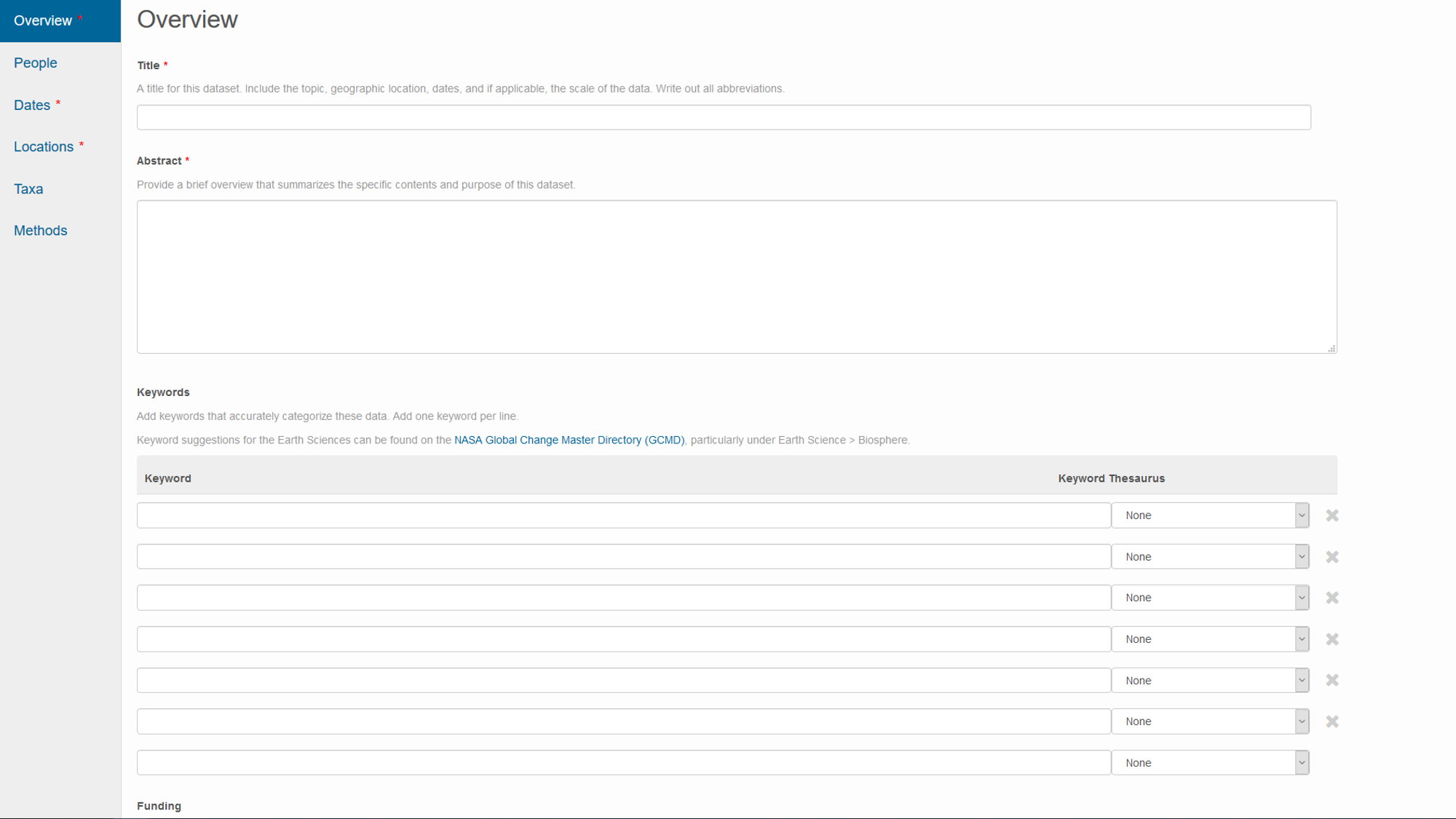
Repository-specific methods
Repository websites frequently guide you through metadata creation during the process of uploading your data.
- website for metadata entry on the Knowledge Network for Biocomplexity repository
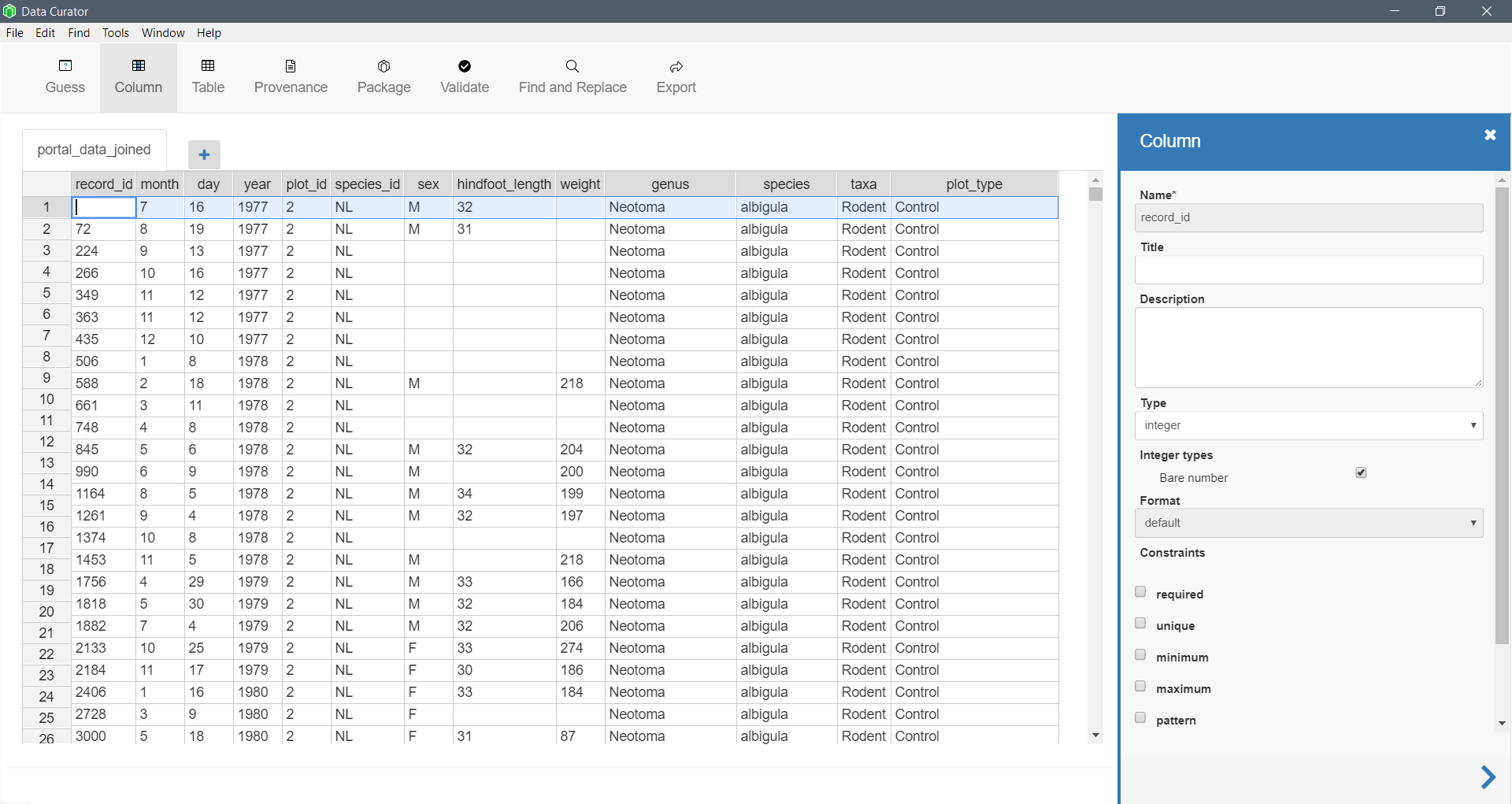
Stand-alone software
Software designed for data curation may have more features and options.
-
Data Curator This software from the Queensland Cyber Infratstructure Foundation supports metadata creation, provenance, and data packaging.
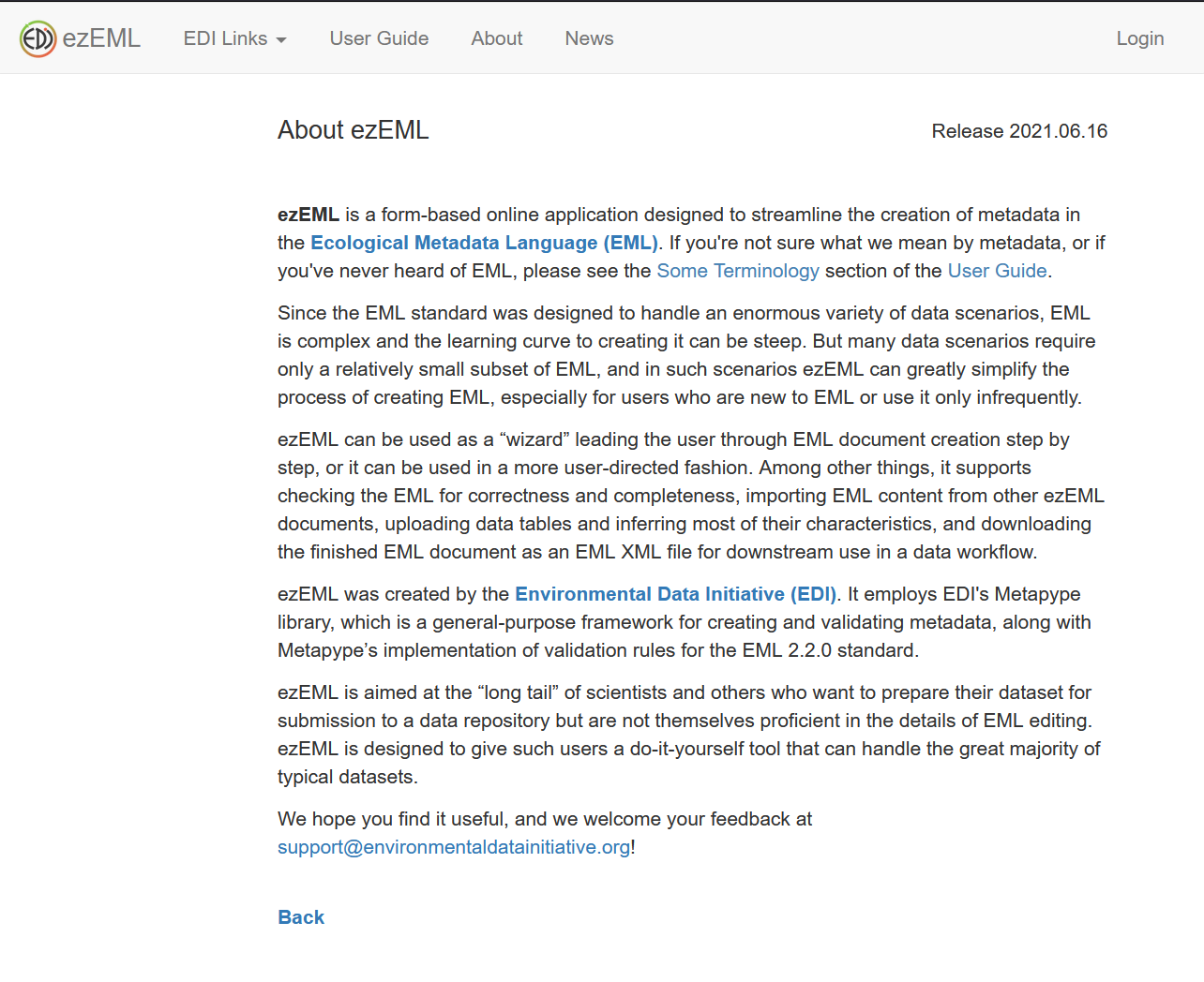
-
ezEML This software from the Environmental Data Initiative supports metadata creation, metadata editing, and multiple metadata co-authors.
Coding
Why would you want to create your metadata programmatically in R? Scripting your metadata creation in R makes updates in the future easier (just update the relevant part of the script and run it), and automating metadata creation is extremely helpful if you are documenting large numbers of data files.
Many methods for documenting and packaging data are also available in R packages developed by repository managers. For example, EMLassemblyline was developed by the Environmental Data Initiative to facilitate documenting data in EML, and preparing data for publication.
- R packages for metadata (EML, dataspice, emld), EMLassemblyline
Example of coding up some metadata
| R Package | What does it do? |
|---|---|
EMLassemblyline |
creates high quality EML metadata for packaging data |
EML |
creates EML metadata files |
We’ll use the EMLassemblyline package to create metadata in the EML metadata standard.
library(EMLassemblyline)
Create the organization for the data package with the EMLassemblyline::template_directories() function.
- data_objects A directory of data and other digital objects to be packaged (e.g. data files, scripts, .zip files, etc.).
- metadata_templates A directory of EMLassemblyline template files.
- eml A directory of EML files created by EMLassemblyline.
- run_EMLassemblyline.R An example R file for scripting an EMLassemblyline workflow. This could be helpful if you’re starting from scratch, but we walk through a metadata workflow in detail below instead.
template_directories(path = "~", dir.name = "storm_project") # create template files in a new directory

# move the derived data file to the new storm_project directory
file.copy("~/StormEvents_d2006.csv", "~/storm_project/data_objects/", overwrite = TRUE)
file.remove("~/StormEvents_d2006.csv")
Look at your storm_project folder, and see the template files and folders, and the derived data file we created earlier.
Describe the package-level metadata.
We’ll start by creating the package-level metadata.
Essential metadata: Create templates for package-level metadata, including abstract, intellectual rights, keywords, methods, personnel, and additional info. These are required for all data packages.
template_core_metadata(path = "~/storm_project/metadata_templates",
                       license = "CCBY",
                       file.type = ".txt")
We’ve chosen the “CCBY” license and the text file type (.txt) because text files are easily read into R and programmatically edited.
You can choose the license you wish to apply to your data (“CC0” or “CCBY”), as well as the file type of the metadata (.txt, .docx, or .md). See the help page for the function for more information. NOTE: The .txt template files are Tab delimited.
Now that the templates have been created, open the files and add the appropriate metadata. They are located in the project directory, the metadata templates folder ~/storm_project/metadata_templates/.
You could open the template files in RStudio and edit manually, or export to Excel and edit there, but let’s read them into R and edit them programmatically. This example can be used to automate the creation of your metadata
We’ll begin by adding a brief abstract.
abs <- "Abstract: Storms can have impacts on people's lives.  These data document some storms in 2006, and the injuries and damage that might have occurred from them."

# this function from the readr package writes a simple text file without columns or rows
write_file(abs, "~/storm_project/metadata_templates/abstract.txt", append = FALSE)
Now we’ll add methods.
methd <- "These example data were generated for the purpose of this lesson.  Their only use is for instructional purposes."

write_file(methd, "~/storm_project/metadata_templates/methods.txt", append = FALSE)
And some add keywords.
NOTE: This must be a 2 column table. You may leave the Thesaurus column empty if you’re not using a controlled vocabulary for your keywords.
keyw <- read.table("~/storm_project/metadata_templates/keywords.txt", sep = "\t", header = TRUE, colClasses = rep("character", 2))

keyw <- keyw[1:3,] # create a few blank rows
keyw$keyword <- c("storm", "injury", "damage") # fill in a few keywords

write.table(keyw, "~/storm_project/metadata_templates/keywords.txt", row.names = FALSE, sep = "\t")
Let’s edit the personnel template file programmatically. NOTE: The .txt template files are Tab delimited.
# read in the personnel template text file
persons <- read.table("~/storm_project/metadata_templates/personnel.txt",
                     sep = "\t", header = TRUE, colClasses = rep("character", 10))

persons <- persons[1:4,] # create a few blank rows

# edit the personnel information
persons$givenName <- c("Jane", "Jane", "Jane", "Hank")
persons$middleInitial <- c("A", "A", "A", "O")
persons$surName <- c("Doe", "Doe", "Doe", "Williams")
persons$organizationName <- rep("University of Maryland", 4)
persons$electronicMailAddress <- c("jadoe@umd.edu", "jadoe@umd.edu", "jadoe@umd.edu", "how@umd.edu")
persons$role <- c("PI", "contact", "creator", "Field Technician")
persons$projectTitle <- rep("Storm Events", 4)
persons$fundingAgency <- rep("NSF", 4)
persons$fundingNumber <- rep("000-000-0001", 4)

# write new personnel file
write.table(persons, "~/storm_project/metadata_templates/personnel.txt", row.names = FALSE, sep = "\t")
IMPORTANT: In the personnel.txt file, if a person has more than one role (for example PI and contact), make multiple rows for this person but change the role on each row. See the help page for the template function for more details.
Geographic coverage: Create the metadata for the geographic extent.
template_geographic_coverage(path = "~/storm_project/metadata_templates",
                             data.path = "~/storm_project/data_objects",
                             data.table = "StormEvents_d2006.csv",
                             lat.col = "BEGIN_LAT",
                             lon.col = "BEGIN_LON",
                             site.col = "STATE"
                             )
Describe the file-level metadata.
Now that we’ve created package-level metadata, we can create the file-level metadata.
Data attributes: Create table attributes template (required when data tables are present)
template_table_attributes(path = "~/storm_project/metadata_templates",
                          data.path = "~/storm_project/data_objects",
                          data.table = c("StormEvents_d2006.csv"))
The template function can’t discover everything, so some columns are still empty. View the file in the metadata templates folder ~/storm_project/metadata_templates/ and enter the missing info.
# read in the attributes template text file
attrib <- read.table("~/storm_project/metadata_templates/attributes_StormEvents_d2006.txt",
                     sep = "\t", header = TRUE)
> View(attrib)
We need to add attribute definitions for each column, and units or date/time specifications for numeric or date/time columns classes.
attrib$attributeDefinition <- c("event id number", "State", "FIPS code for state", "year",
                                "month", "type of event", "date event started", "timezone",
                                "date event ended", "injuries as direct result of storm",
                                "injuries as indirect result of storm",
                                "deaths - direct result", "deaths - indirect result",
                                "property damage", "crop damage", "source of storm info",
                                "manitude of damage", "type of magnitude",
                                "beginning latitude", "beginning longitude", "ending latitude",
                                "ending longitude", "narrative of the episode",
                                "narrative of the event", "source of the data")

attrib$dateTimeFormatString <- c("","","","YYYY","","","MM/DD/YYYY HH:MM",
                                 "three letter time zone","MM/DD/YYYY HH:MM",
                                 "","","","","","","","","","","","","","","","")
It is also important to define missing value codes. This is frequently NA, but should still be defined explicitly.
attrib$missingValueCode <- rep(NA_character_, nrow(attrib))

attrib$missingValueCodeExplanation <- rep("Missing value", nrow(attrib))
In addition, it’s good to double check the class of variables inferred by the templating function. In this case, we’ve decided four variables would be better described as character rather than categorical.
attrib$class <- attrib %>% select(attributeName, class) %>%
                mutate(class = ifelse(attributeName %in% c("DAMAGE_PROPERTY", "DAMAGE_CROPS",
                                                           "EVENT_TYPE", "SOURCE"),
                                      "character", class)) %>%
                select(class) %>% unlist(use.names = FALSE)
Units need to be defined from a controlled vocabulary of standard units. Use the function view_unit_dictionary() to view these standard units.
If you can’t find your units here, they must be defined in the file custom_units.txt in the metadata templates folder. Generally, if you are not comfortable with a definition then it is best to provide a custom unit definition. There are some non-intuitive definitions, such as using the broad unit “degree” for latitude and longitude such as in our example data here.
> view_unit_dictionary()
attrib$unit <- c("number","","number","","","","","","","number","number","number",
                 "number","","","","number","","degree",
                 "degree","degree","degree","","","")
Check your edits are all correct.
> View(attrib)
Now we can write out the attribute file we just edited.
write.table(attrib, "~/storm_project/metadata_templates/attributes_StormEvents_d2006.txt", row.names = FALSE, sep = "\t")
Because we have categorical variables in our data file, we need to define those variables further using the following templating function.
Categorical variables: Create metadata specific to categorical variables (required when the attribute metadata contains variables with a “categorical” class)
template_categorical_variables(path = "~/storm_project/metadata_templates",
                               data.path = "~/storm_project/data_objects")
$catvars_StormEvents_d2006.txt
$catvars_StormEvents_d2006.txt$content
    attributeName           code definition
1     DATA_SOURCE            CSV
2     DATA_SOURCE            PDS
3  MAGNITUDE_TYPE             EG
4  MAGNITUDE_TYPE             MG
5      MONTH_NAME          April
6      MONTH_NAME       February
7      MONTH_NAME        January
8      MONTH_NAME        October
9           STATE         ALASKA
10          STATE       ARKANSAS
11          STATE       COLORADO
12          STATE        GEORGIA
13          STATE       ILLINOIS
14          STATE        INDIANA
15          STATE         KANSAS
16          STATE       KENTUCKY
17          STATE      LOUISIANA
18          STATE       MARYLAND
19          STATE       MICHIGAN
20          STATE     NEW JERSEY
21          STATE NORTH CAROLINA
22          STATE           OHIO
23          STATE       OKLAHOMA
24          STATE          TEXAS
25          STATE           UTAH
26          STATE     WASHINGTON
27          STATE  WEST VIRGINIA
Define categorical variable codes.
NOTE: You must add definitions, even for obvious things like month. If you don’t add definitions, your EML metadata will be invalid.
# read in the attributes template text file
catvars <- read.table("~/storm_project/metadata_templates/catvars_StormEvents_d2006.txt",
                      sep = "\t", header = TRUE)

catvars$definition <- c("csv file", "pds file", rep("magnitude", 2), rep("month", 4), rep("USA state", 19))

write.table(catvars, "~/storm_project/metadata_templates/catvars_StormEvents_d2006.txt", row.names = FALSE, sep = "\t")
NOTE: If you have not filled in the table attributes template completely, the template_categorical_variables() function may produce errors. It also produces a useful warning message that you can use to look at the issues.
If you type issues() in your R console, you’ll get helpful info on which issues you need to fix.
> issues()
Write EML metadata file
Many repositories for environmental data use EML (Ecological Metadata Language) formatting for metadata. The function make_eml() converts the text files we’ve been editing into EML document(s).
Check the function help documentation to see which arguments of make_eml() are required and which are optional.
make_eml(path = "~/storm_project/metadata_templates",
         data.path = "~/storm_project/data_objects",
         eml.path = "~/storm_project/eml",
         dataset.title = "Storm Events that occurred in 2006",
         temporal.coverage = c("2006-01-01", "2006-04-07"),
         geographic.description = "Continental United State of America",
         geographic.coordinates = c(30, -79, 42.5, -95.5),
         maintenance.description = "In Progress: Some updates to these data are expected",
         data.table = "StormEvents_d2006.csv",
         data.table.name = "Storm_Events_2006",
         data.table.description = "Storm Events in 2006",
         # other.entity = c(""),
         # other.entity.name = c(""),
         # other.entity.description = c(""),
         user.id = "my_user_id",
         user.domain = "my_user_domain",
         package.id = "storm_events_package_id")
This function tries to validate your metadata against the EML standard. If there are problems making your metadata invalid, type issues() into your console (as above), and you’ll receive useful information on how to make your metadata valid.
After you create your EML file, it might be useful to double check it. EML isn’t very human-readable, so try using the online Metadata Previewer tool from the Environmental Data Initiative for viewing your EML.
Packaging your data
Data packages can include metadata, data, and script files, as well as descriptions of the relationships between those files.
Packaging your data together with the code you used to make the data file, and the metadata that describes the data, can benefit you and your research team because it keeps this information together so you can more easily share it, and it will be ready to publish (perhaps with minor updates if you wish) when you are ready.
Currently there are a few ways to make a data package:
- Frictionless Data uses json-ld format, and has the R package
datapackage.rwhich creates metadata files using schema.org specifications and creates a data package.
- DataONE frequently uses EML format for metadata, and has related R packages
datapackanddataonethat create data packages and upload data packages to a repository.
We’ll follow the DataONE way of creating a data package in this lesson.
| R Package | What does it do? |
|---|---|
datapack |
creates data package including file relationships |
uuid |
creates a unique identifier for your metadata |
Data, Metadata, and other objects
We’ll create an empty local data package using the new() function from the datapack: R package.
library(datapack)
library(uuid)

dp <- new("DataPackage") # create empty data package
Add the metadata file we created earlier to the blank data package.
emlFile <- "~/storm_project/eml/storm_events_package_id.xml"
emlId <- paste("urn:uuid:", UUIDgenerate(), sep = "")

mdObj <- new("DataObject", id = emlId, format = "eml://ecoinformatics.org/eml-2.1.1", file = emlFile)

dp <- addMember(dp, mdObj)  # add metadata file to data package
Add the data file we saved earlier to the data package.
datafile <- "~/storm_project/data_objects/StormEvents_d2006.csv"
dataId <- paste("urn:uuid:", UUIDgenerate(), sep = "")

dataObj <- new("DataObject", id = dataId, format = "text/csv", filename = datafile)

dp <- addMember(dp, dataObj) # add data file to data package
Define the relationship between the data and metadata files. The “subject” should be the metadata, and the “object” should be the data.
# NOTE: We have defined emlId and dataId in the code chunks above.
dp <- insertRelationship(dp, subjectID = emlId, objectIDs = dataId)
You can also add scripts and other files to the data package. Let’s add a short script to our data package, as well as the two figures it creates.
scriptfile <- "data/storm_script.R"
scriptId <- paste("urn:uuid:", UUIDgenerate(), sep = "")

scriptObj <- new("DataObject", id = scriptId, format = "application/R", filename = scriptfile)

dp <- addMember(dp, scriptObj)
fig1file <- "data/Storms_Fig1.png"
fig1Id <- paste("urn:uuid:", UUIDgenerate(), sep = "")

fig1Obj <- new("DataObject", id = fig1Id, format = "image/png", filename = fig1file)

dp <- addMember(dp, fig1Obj)
fig2file <- "data/Storms_Fig2.png"
fig2Id <- paste("urn:uuid:", UUIDgenerate(), sep = "")

fig2Obj <- new("DataObject", id = fig2Id, format = "image/png", filename = fig2file)

dp <- addMember(dp, fig2Obj)
Provenance
Provenance defines the relationships between data, metadata, and other research objects (inputs and outputs) generated throughout the research process, from raw data to publication(s). It can be recorded in several different formats, but we’ll explore a couple here.
Resource Description Framework (RDF) describes links between objects, and is designed to be read and understood by computers. RDF is not designed to be read by humans, and is written in XML. Describing your data package relationships with RDF will help with displaying your data in an online repository. If you’re interested in the details, you can read more online such as from w3.
We’ll create a Resource Description Framework (RDF) to define the relationships between our data and metadata in XML.
serializationId <- paste("resourceMap", UUIDgenerate(), sep = "")
filePath <- file.path(sprintf("%s/%s.rdf", tempdir(), serializationId))
status <- serializePackage(dp, filePath, id = serializationId, resolveURI = "")
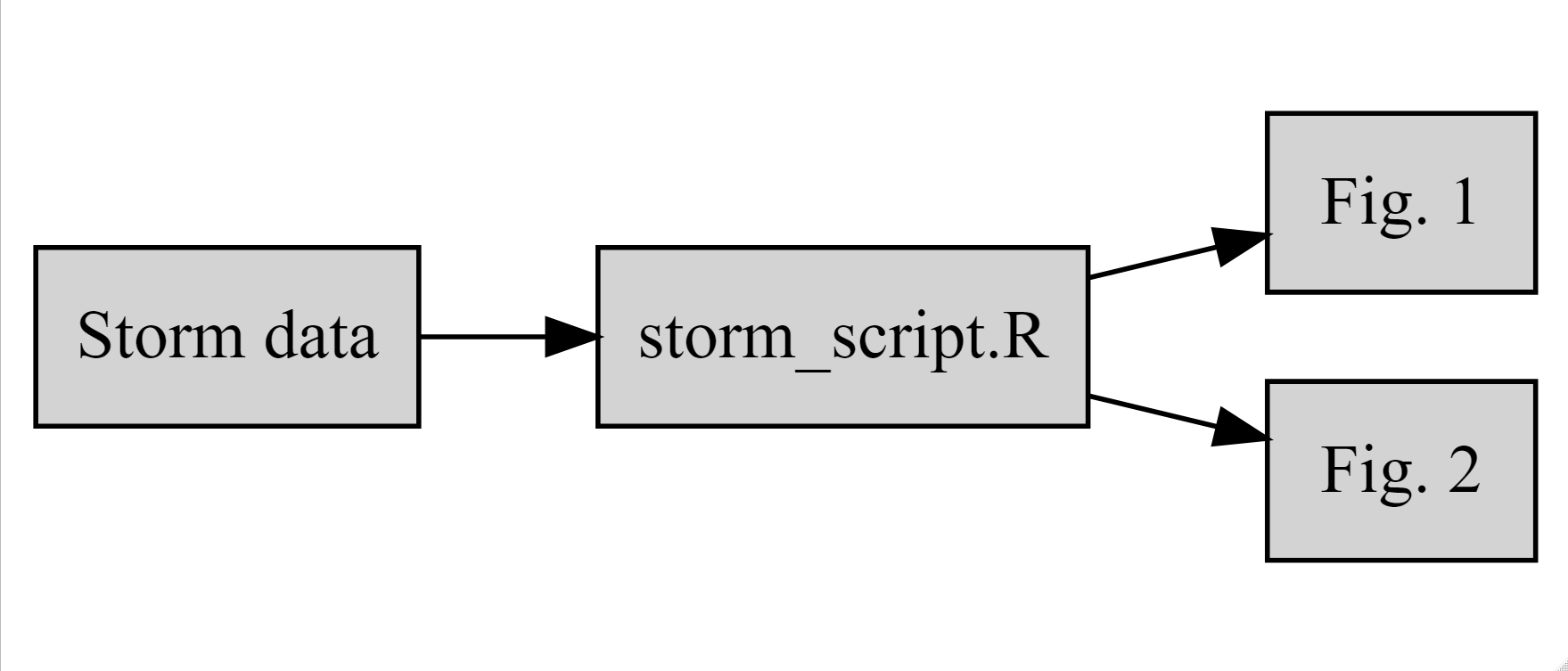
When thinking about the relationships between your data, metadata, and other objects, it is often very helpful to create a diagram. Here an couple example:
-
simple path diagram
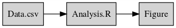
Let’s create a conceptual diagram of the relationships between our data, script, and figures.
library(DiagrammeR)

storm_diag <- grViz("digraph{

                     graph[rankdir = LR]

                     node[shape = rectangle, style = filled]
                     A[label = 'Storm data']
                     B[label = 'storm_script.R']
                     C[label = 'Fig. 1']
                     D[label = 'Fig. 2']

                     edge[color = black]
                     A -> B
                     B -> C
                     B -> D

                     }")

storm_diag
Adding the provenance to your data package
Human-readable provenance can be added to a data package using datapack and the function describeWorkflow, as in the example code below.
See the overview or the function documentation for more details.
We’ll define the relationship between our data, our script that creates 2 figures, and our figures.
# NOTE: we defined the objects here in the code above
dp <- describeWorkflow(dp, sources = dataObj, program = scriptObj, derivations = c(fig1Obj, fig2Obj))
Now let’s take a look at those relationships we just defined.
library(igraph)
plotRelationships(dp)
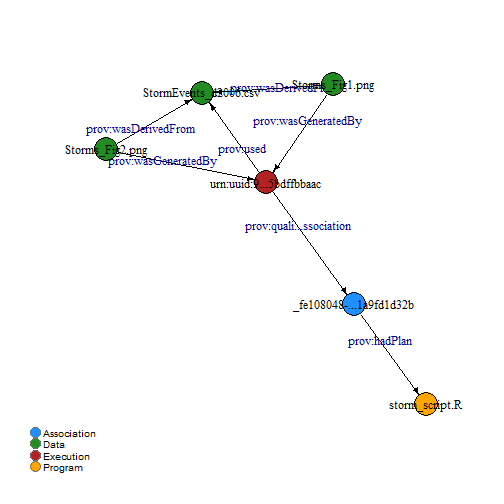
Why does the diagram we created above differ from the provenance diagram created by the function datapack::describeWorkflow? The datapack function adds additional descriptive nodes to the diagram that fulfill certain semantic requirements. However, the basic relationships are still there if you look carefully.
Save the data package to a file, using the BagIt packaging format.
Right now this creates a zipped file in the tmp directory. We’ll have to move the file out of the temp directory after it is created. Hopefully this will be changed soon!
dp_bagit <- serializeToBagIt(dp)

file.copy(dp_bagit, "~/storm_project/Storm_data_package.zip")
[1] TRUE
The BagIt zipped file is an excellent way to share all of the files and metadata of a data package with a collaborator, or easily publish in a repository.
Publishing your data
Now that you’ve packaged up your data, it’s easier to publish!
Choosing to publish your data in a long-term repository can:
- enable versioning of your data
- fulfill a journal requirement to publish data
- facilitate citing your dataset by assigning a permanent uniquely identifiable code (DOI)
- improve discovery of and access to your dataset for others
- enable re-use and greater visibility of your work
Why can’t I just put my data on Dropbox, Google Drive, my website, etc?

Key reasons to use a repository:
- preservation (permanence)
- stability (replication / backup)
- access
- standards
When to publish your data?
Near the beginning? At the very end?
A couple issues to think about:
1) How do you know you’re using the same version of a file as your collaborator?
- Publish your data privately and use the unique ids of datasets to manage versions.
2) How do you control access to your data until you’re ready to go public with it?
- Embargoing - controlling access for a certain period of time and then making your data public.
Get an ORCiD
ORCiDs identify you and link you to your publications and research products. They are used by journals, repositories, etc. and often as a log in.
If you don’t have one yet, get an ORCiD. Register at https://orcid.org.

Picking a repository
There are many repositories out there, and it can seem overwhelming picking a suitable one for your data.
Repositories can be subject or domain specific. re3data lists repositories by subject and can help you pick an appropriate repository for your data.
DataONE is a federation of repositories housing many different types of data. Some of these repositories include Knowledge Network for Biocomplexity (KNB), Environmental Data Initiative (EDI), Dryad, USGS Science Data Catalog
For qualitative data, there are a few dedicated repositories: QDR, Data-PASS
Though a bit different, Zenodo facilitates publishing (with a DOI) and archiving all research outputs from all research fields.
One example is using Zenodo to publish releases of your code that lives in a GitHub repository. However, since GitHub is not designed for data storage and is not a persistent repository, this is not a recommended way to store or publish data.
Uploading to a repository
Uploading requirements can vary by repository and type of data. The minimum you usually need is basic metadata, and a data file.
If you have a small number of files, using a repository GUI may be simpler. For large numbers of files, automating uploads from R will save time. And it’s reproducible, which is always good!
Data Upload Example - DataONE:
If you choose to upload your data package to a repository in the DataONE federation of repositories, the following example may be helpful. The basic steps we will walk through in detail below are
1) Getting an authentication token (follow steps below)
2) Getting a DOI (if desired) from your chosen repository
3) Uploading your data package using R
| R Package | What does it do? |
|---|---|
dataone |
uploads data package to repository |
library(dataone)
library(curl)
library(redland)
Tokens:
Different environments in DataONE take different authentication tokens. Essentially, the staging environment is for testing, and the production environment is for publishing. If you are running the code in this lesson with the example data included here, get a token for the staging environment. If you are modifying this code to publish your own research data, get a token for the production environment.
To get a token for the staging environment start here Staging Environment.
To get a token for the production environment start here Production Environment.
If you happen to notice that the staging environment link above is an address at nceas.ucsb.edu, don’t worry. DataONE is a project administered by NCEAS, which is a research affiliate of UCSB.
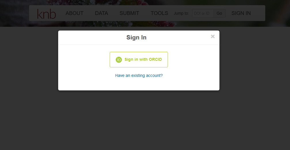
After following either link above, complete the following steps to get your token.
- Click Sign in, or Sign up if necessary
- Once signed in, move the cursor over the user name and select My profile in the drop down menu.
- Click on the Settings tab.
- Click on Authentication Token in the menu below Welcome
- Click on the Token for DataONE R tab.
- Click Renew authentication token if the token you have been using has expired.
- Click on the Copy button below the text window to copy the authentication string to the paste buffer.
- Paste the token string in the R console.
You may want to note the expiration date of the token, which will be displayed on this page.
Set your token now
Paste your token for DataONE R in the R console, as stated in the instructions above.
Citation
Getting a Digital Object Identifier (DOI) for your data package can make it easier for others to find and cite your data.
DOIs are associated with a particular repository or publisher, so you will need to specify the environment and repository (also called a member node) in which you are publishing your data.
The environment is where you publish your data: “PROD” is production, and “STAGING” is to test uploading your data, and can be used if you’re not yet sure you have everything in order.
NOTE: “PROD” and “STAGING” require different tokens.
See above steps to get the appropriate access token.
If you don’t know your repository specs, look it up in this table of member node IDs: (data/Nodes.csv)
read.csv("data/Nodes.csv")
You can get a DOI from your target repository if you desire. We won’t actually do this in the lesson here, because we’re not going to publish our example data. However, this code is provided for your future use when you are ready to publish your own data with a DOI.
# cn <- CNode("PROD")
# mn <- getMNode(cn, "urn:node:KNB")

# doi <- generateIdentifier(mn, "DOI")
Then you would overwrite the previous metadata file with the new DOI identified metadata file. Again, we won’t do this here, as we’re not going to publish our example data. But the code provided here can be modified when you are ready to publish your own data.
# emlFile <- "~/storm_project/eml/storm_events_package_id.xml"

# mdObj <- new("DataObject", id = doi, format = "eml://ecoinformatics.org/eml-2.1.1", file = emlFile)

# dp <- addMember(dp, mdObj)
Then you would zip up all your files for your data package with BagIt as shown in the previous section.
Set access rules
NOTE: Replace this example ORCID with your own ORCID!
dpAccessRules <- data.frame(subject = "http://orcid.org/0000-0003-0847-9100",
                            permission = "changePermission")
This gives this particular ORCID (person) permission to read, write, and change permissions for others for this package.
dpAccessRules2 <- data.frame(subject = c("http://orcid.org/0000-0003-0847-9100",
                                         "http://orcid.org/0000-0000-0000-0001"),
                             permission = c("changePermission", "read")
                             )
The second person (ORCID) only has access to read the files in this package.
NOTE: When you upload the package, you can set public = FALSE if you don’t want your package public yet.
Upload data package
First set the environment and repository you’ll upload to.
NOTE: We are using the “STAGING2” environment and “TestKNB” repository node here, because we just want to test uploading, but not actually publish our example data package.
d1c <- D1Client("STAGING2", "urn:node:mnTestKNB")
Now do the actual uploading of your data package to the test repository location.
packageId <- uploadDataPackage(d1c, dp, public = TRUE, accessRules = dpAccessRules,
                               quiet = FALSE)
Versioning Data
How do you know you’re using the same version of a data file as your collaborator?
- Do not edit raw data files! Make edits/changes via your code only, and then output a derived “clean” data file.
Potential ways forward:
-
Upload successive versions of the data to a repo with versioning, but keep it private until you’ve reached the final version or the end of the project. (see below)
-
Google Sheets has some support for viewing the edit history of cells, added or deleted columns and rows, changed formatting, etc.
Updating your data package on the repository
To take advantage of the versioning of data built into many repositories, you can update the data package (replace files with new versions).
Please see the vignettes for dataone , in the section on “Replace an object with a newer version”.
It’s also possible to automate data publication for data that are updated periodically, such as monitoring data, or time-series data. The R package EMLassemblyline has a vignette describing the process.
Closing thoughts
Starting to document your data at the beginning of your project will save you time and headache at the end of your project.
Integrating data documentation and publication into your research workflow will increase collaboration efficiency, reproducibility, and impact in the science community.
Exercises
Exercise 1
ORCiDs identify you (like a DOI identifies a paper) and link you to your publications and research products.
If you don’t have an ORCiD, register and obtain your number at https://orcid.org.
Exercise 2
The DataONE federation of repositories requires a unique authentication token for you to upload a data package.
Follow the steps here to obtain your token.
Exercise 3
There are many repositories you could upload your data package to within the DataONE federation.
Pick a repository from the list (located at data/Nodes.csv) and upload a test data package to the “STAGING” environment.
Note: Staging environments require a different authentication token than production environments. See the section on token in the publishing part of the lesson for more details.
Exercise 4
DOIs (digital object identifiers) are almost univerally used to identify papers. They also improve citation and discoverability for your published data packages.
Get a DOI for your published data package.
Exercise 5
If you’re using a data repository to manage versions of your derived data files, you will likely want to update your data file at some point. Use the vignette from the dataone package to “replace an older version of your derived data” with a newer version.
Exercise 6
Provenance is an important description of how your data have been obtained, cleaned, processed, and analyzed. It is being incorporated into descriptions of data packages in some repositories.
Use the describeWorkflow() function from the datapack package to add provenance to your test data package.
If you need to catch-up before a section of code will work, just squish it's 🍅 to copy code above it into your clipboard. Then paste into your interpreter's console, run, and you'll be ready to start in on that section. Code copied by both 🍅 and 📋 will also appear below, where you can edit first, and then copy, paste, and run again.
# Nothing here yet!