Pipelines for Online Data
USGS FEWS NET Data Portal
Lesson 7 with Ian Carroll
Contents
Objectives for this lesson
- Access data from a web service
- Start a data “analysis” pipeline
- Meet rasterio, for geospatial arrays
Specific achievements
- Script aquistion from a NASA data portal
- Get just the data you need with OPeNDAP
- Mask rasters with shapefiles in Python
Drought Monitoring
The NOAA Climate Prediction Center provides forecasts to assist USAIDs food security programs.
In the report dated March 29 – April 4, 2018, moisture deficits shown for regions of southern Africa and Madagascar are inferred from regularly updated land surface models. The NASA program that maintains those products, the Famine Early Warning Systems Network Land Data Assimilation System (FLDAS), also distributes them through the EARTHDATA portal.
The latest report suggests trouble in the Limpopo basin.
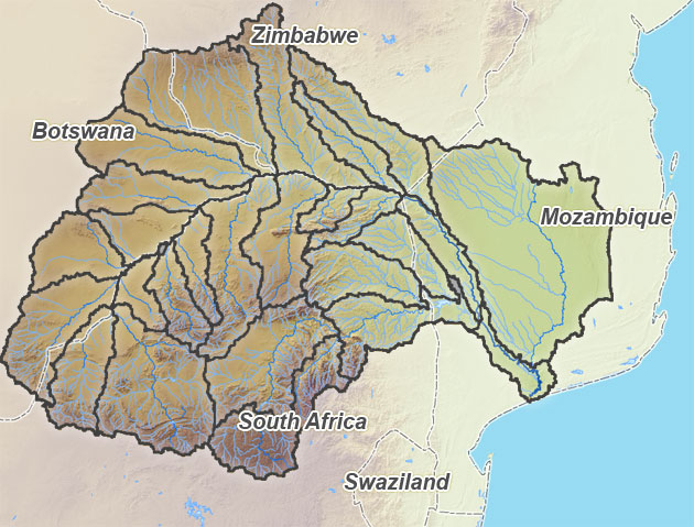
Credit: River Awareness Kit
EARTHDATA
The NASA EARTHDATA site provides web access to the Earth Observing System Data and Information System (EOSDIS), which distributes products from multiple missions to users.
- Register for an Earthdata Login.
- Use the following in a terminal to create a “~/.netrc” file:
echo "machine urs.earthdata.nasa.gov" > ~/.netrc
echo "login ... " >> ~/.netrc
echo "password ..." >> ~/.netrc
chmod 600 ~/.netrc
Search for “FLDAS” datasets. Can you find a link to the data? The more comprehensive the data portal, the more opaque the interface. The data archivers (the DAACs) each provide their own portals for the data they archive, with more specific access instructions application.
Each DAAC requires it’s own “authorization” using your EARTHDATA login, described on the User Registration help page.
GES DISC
Narrow down the FLDAS datasets within the GES DISC.
Filter to:
- 0.1 x 0.1 degree
- Monthly
Select the Anomaly data for Southern Africa modeled with the Noah LSM.
The GES DISC portal provides large temporal and spatial extents. We have established the narrower task of investigating evidence of drought in the Limpopo basin.
- Use the GUI to subset the resource (good once).
- Script data aquistion for a reproducible and reusable pipeline.
OPeNDAP Server/Client
The GES DISC provides access through a web service called OPeNDAP. The OPenDAP server is listening for requests at a URL, just like a website server.
dap = 'https://hydro1.gesdisc.eosdis.nasa.gov/opendap/hyrax/FLDAS/'
resource = 'FLDAS_NOAH01_C_SA_MA.001/2013/FLDAS_NOAH01_C_SA_MA.ANOM201301.001.nc'
url = dap + resource
Some portals, GES DISC is one, require authentication to access the data, whether you use the GUI or request it programatically.
from netrc import netrc
username, _, password = netrc().hosts['urs.earthdata.nasa.gov']
The OPeNDAP server’s response is not a website. We need a OPeNDAP client to handle the response.
from pydap.client import open_url
from pydap.cas.urs import setup_session

session = setup_session(username, password, check_url = url)
dataset = open_url(url, session = session)
dataset.keys()
Out[1]: KeysView(<DatasetType with children 'lon', 'lat', 'time', 'time_bnds', 'SoilMoi00_10cm_tavg', 'SoilMoi10_40cm_tavg', 'SoilMoi40_100cm_tavg', 'SoilMoi100_200cm_tavg', 'Evap_tavg', 'Rainf_f_tavg', 'Tair_f_tavg', 'Qtotal_tavg'>)
Your client is ready to request variables from this dataset. All OPeNDAP data follows a standard data model (very similar to netCDF4 model) and is independent of how GES DISC stores the data.
varname = 'SoilMoi10_40cm_tavg'
variable = dataset[varname]
variable.shape
Out[1]: (1, 443, 486)
The data array is transmitted along with the dimensions ordered as (bands, rows, columns). In this call, we get all bands (there’s only one), the first two rows, and the first three columns.
variable[:, :2, :3].data
Out[1]:
[array([[[-9999., -9999., -9999.],
         [-9999., -9999., -9999.]]], dtype=float32),
 array([ 11323.]),
 array([-37.85, -37.75]),
 array([ 6.05,  6.15,  6.25])]
The variable.shape is not huge, so get all the data. Our current objective is to figure out how to script the aquisition of a subset, and we don’t want to harass the server while we hack about.
var = variable[:, :, :]
var[:, :2, :3].data
Out[1]:
[array([[[-9999., -9999., -9999.],
         [-9999., -9999., -9999.]]], dtype=float32),
 array([ 11323.]),
 array([-37.85, -37.75]),
 array([ 6.05,  6.15,  6.25])]
The dataset and variable objects provide all the values and critical metadata.
data = var.array.data
dims = {k: v.data for k, v in var.maps.items()}
nodata = dataset.attributes['NC_GLOBAL']['missing_value']
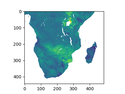
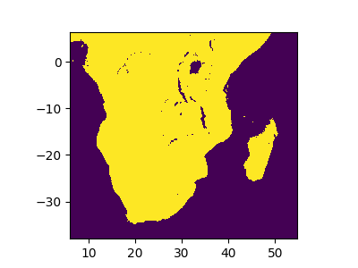
import matplotlib.pyplot as plt
plt.imshow(data[0, :, :])
Out[1]: <matplotlib.image.AxesImage at 0x7f3bbae10278>
Data Alignment
The var.array.data attribute is a numpy array, allowing for some needed adjustments.
import numpy as np

data = np.flip(data, 1).astype('float32')
nodata = data.dtype.type(nodata)
The rasterio package provides an interface to GDAL/OGR and PROJ4 for georeferencing the numpy’s numerical arrays.
from rasterio import open as raster

meta = {
    'driver': 'GTiff',
    'dtype': data.dtype,
    'count': data.shape[0],
    'height': data.shape[1],
    'width': data.shape[2],
    'nodata': nodata,
}
with raster(varname + '.tif', 'w', **meta) as r:
    r.write(data[0, :, :], 1)
from rasterio.plot import show

with raster(varname + '.tif') as r:
    show(r.read(1, masked = True))
The warnings arise from the lack of a CRS and extent, or more generally an affine transform.
from rasterio.crs import CRS
from rasterio.transform import from_origin

crs = CRS.from_epsg(4326) # a guess!
attr = dataset.attributes['NC_GLOBAL']
transform = from_origin(
    dims['lon'][0].item(), # west
    dims['lat'][-1].item(), # north (flip!)
    attr['DX'], # xsize
    attr['DY']) # ysize
Update the metadata to include a CRS and the transform, then write to file.
meta.update({
    'crs': crs,
    'transform': transform,
})
with raster(varname + '.tif', 'w', **meta) as r:
    r.write(data[0, :, :], 1)
Now rasterio recognizes use the georeferencing when showing the image.
with raster(varname + '.tif') as r:
    show((r, 1))
More importantly, we can overlay a shapefile in the same CRS to mask the Limpopo basin.
import geopandas as gpd
fig, ax = plt.subplots()

basin = gpd.read_file(
    '/data/Aqueduct_river_basins_LIMPOPO')
with raster(varname + '.tif') as r:
    show((r, 1), ax = ax)
basin.plot(ax = ax,
    color='none', edgecolor = 'black')
Out[1]: <matplotlib.axes._subplots.AxesSubplot at 0x7f3b98fd2400>

fig
Out[1]: <matplotlib.figure.Figure at 0x7f3bac04b828>
Subsetted Requests
The OPeNDAP server allows us to subset the request for data, as opposed to requesting data and then subsetting. Create such a request by subsetting variable. Recall that variable is a connection to the server, not a numpy array.
But what is the subset? It is the window of the raster matching the extent of the polygon. We also want to mask out any remaining pixels outisde the basin. The mask() utility will accomplish both.
from rasterio.mask import mask
from shapely.geometry import mapping

feature = [mapping(g) for g in basin['geometry']]
with raster(varname + '.tif') as r:
    masked, transform = mask(r, feature)
    meta = r.meta.copy()
Write the masked data to a new file, using the original metadata.
with raster(varname + '_basin.tif', 'w', **meta) as r:
    r.write(masked)
The file we just wrote will be the source of the critical information we need for our pipeline: both the window around the basin and the explit mask around the basin.
from rasterio.windows import get_data_window

with raster(varname + '_basin.tif') as r:
    var = r.read(1, masked = True)

y, x = get_data_window(var)
basin = var.mask[slice(*y), slice(*x)]
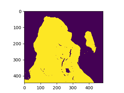
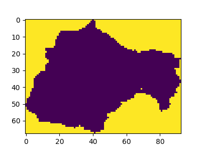
Slicing the mask with y and x reduce the mask to same shape as the data subset we are going to request.
show(basin)
Out[1]: <matplotlib.axes._subplots.AxesSubplot at 0x7f3bbadc2c18>
Statistics calculated on a masked variable refer only to the pixesl within the basin.
type(var), var.mean()
Out[1]: (numpy.ma.core.MaskedArray, 0.028327035785673998)
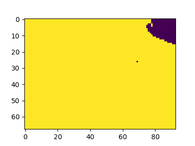
While the x and y variables provide the slices we want to request, don’t forget to acconut for flipping the y-axis.
y = variable.shape[1] - y[1], variable.shape[1] - y[0]
var = variable[:, slice(*y), slice(*x)]
show(var)
Out[1]: <matplotlib.axes._subplots.AxesSubplot at 0x7f3b8c67de48>
Loop though Time
Finally, we have everything we need to build a time series of basin means.
- a
sessionto contact the server - a time-varying resource to request
- a window to request with
- a basin mask the same size as the window
from pandas import Series
basin_ts = Series(index = [[],[]])

name = 'FLDAS_NOAH01_C_SA_MA'
resource = '{0}.001/{1}/{0}.ANOM{1}{2:02d}.001.nc'

yr = 2016
mo = 0
while True:

    # connect to resource
    # for year and month
    url = dap + resource.format(name, yr, mo + 1)
    try:
        dataset = open_url(url,
            session = session)
    except:
        break

    # request data subset
    # and store masked mean
    variable = dataset[varname]
    var = variable[:, slice(*y), slice(*x)]
    data = np.flip(var.array.data, 1)
    data = np.ma.array(
        data,
        mask = basin)
    basin_ts[yr, mo + 1] = data.mean()

    # increment month and year
    mo = (mo + 1) % 12
    yr = yr + 1 if mo == 0 else yr

basin_ts.to_pickle('basin_ts.pickle')
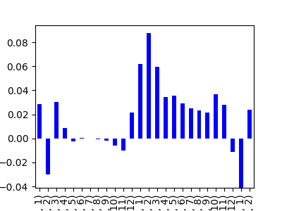
Plot a simple bar chart to see how soil moisture anomolies have varied between months over the past couple years.
basin_ts.plot.bar(color = 'b')
Out[1]: <matplotlib.axes._subplots.AxesSubplot at 0x7f3b8c5f2208>