Vector and Raster Geospatial Data
Lesson 7 with Quentin Read
Lesson Objectives
- Meet the key R packages for geospatial analysis
- Learn basic wrangling of vector and raster data
- Distinguish “scriptable” tasks from desktop GIS tasks
Specific Achievements
- Create, load, and plot vector data types, or “features”
- Filter features based on associated data or on spatial location
- Perform geometric operations on polygons
- Load, manipulate, and extract raster data
R Packages
The key R packages for this lesson are
OSGeo Dependencies
Most R packages depend on other R packages. The sf and raster packages also depend on system libraries.
- GDAL for read/write in geospatial data formats
- GEOS for geometry operations
- PROJ.4 for cartographic projections
System libraries cannot be installed by R’s install.packages(), but can be
bundled with these packages and for private use by them. Either way, the
necessary libraries are maintained by the good people at the Open Source
Geospatial Foundation for free and easy distribution.
Vector Data
The US Census website distributes county polygons (and much more) that are provided with the handouts. The sf package reads shapefiles (“.shp”) and most other vector data:
library(sf)

shp <- 'data/cb_2016_us_county_5m'
counties <- st_read(
  shp,
  stringsAsFactors = FALSE)
The counties object is a data.frame that includes a sfc, which stands for
“simple feature column”. This special column is usually called “geometry” or
“geom” (not to be confused with ggplot’s geoms)!
> head(counties)
Simple feature collection with 6 features and 9 fields
geometry type:  MULTIPOLYGON
dimension:      XY
bbox:           xmin: -114.7556 ymin: 29.26116 xmax: -81.10192 ymax: 38.77443
CRS:            4269
  STATEFP COUNTYFP COUNTYNS       AFFGEOID GEOID      NAME LSAD       ALAND
1      04      015 00025445 0500000US04015 04015    Mohave   06 34475567011
2      12      035 00308547 0500000US12035 12035   Flagler   06  1257365642
3      20      129 00485135 0500000US20129 20129    Morton   06  1889993251
4      28      093 00695770 0500000US28093 28093  Marshall   06  1828989833
5      29      510 00767557 0500000US29510 29510 St. Louis   25   160458044
6      35      031 00929107 0500000US35031 35031  McKinley   06 14116799068
     AWATER                       geometry
1 387344307 MULTIPOLYGON (((-114.7556 3...
2 221047161 MULTIPOLYGON (((-81.52366 2...
3    507796 MULTIPOLYGON (((-102.042 37...
4   9195190 MULTIPOLYGON (((-89.72432 3...
5  10670040 MULTIPOLYGON (((-90.31821 3...
6  14078537 MULTIPOLYGON (((-109.0465 3...
Geometry Types
Like any data.frame column, the geometry column is comprised of a single
data type. The “MULTIPOLYGON” is just one of several standard geometric data
types.
| Common Types | Description |
|---|---|
| POINT | zero-dimensional geometry containing a single point |
| LINESTRING | sequence of points connected by straight, non-self intersecting line pieces; one-dimensional geometry |
| POLYGON | sequence of points in closed, non-intersecting rings; the first denotes the exterior ring, any subsequent rings denote holes |
| MULTI* | set of * (POINT, LINESTRING, or POLYGON) |
The spatial data types are built upon each other in a logical way: lines are built from points, polygons are built from lines, and so on.
We can create any of these spatial objects from coordinates.
Here’s an sfc object with a single “POINT”, corresponding to SESYNC’s position
in WGS84 degrees latitude and degrees longitude, with the same coordinate
reference system as the counties object.
sesync <- st_sfc(st_point(
    c(-76.503394, 38.976546)),
    crs = st_crs(counties))
Coordinate Reference Systems
A key feature of a geospatial data type is its associated CRS, stored as an
EPSG ID and an equivalent PROJ.4 string. We can print the CRS of a spatial
object with st_crs().
> st_crs(counties)
Coordinate Reference System:
  User input: 4269
  wkt:
GEOGCS["GCS_North_American_1983",
    DATUM["North_American_Datum_1983",
        SPHEROID["GRS_1980",6378137,298.257222101]],
    PRIMEM["Greenwich",0],
    UNIT["Degree",0.017453292519943295],
    AUTHORITY["EPSG","4269"]]
Bounding Box
A bounding box for all features in an sf data frame is generated by st_bbox().
> st_bbox(counties)
      xmin       ymin       xmax       ymax
-179.14734  -14.55255  179.77847   71.35256
The bounding box is not a static attribute—it is determined on-the-fly for the entire table or any subset of features. In this example, we subset the United States counties by state ID 24 (Maryland).
Because the counties object is a kind of data.frame, we can use dplyr
verbs such as filter on it, just as we would with a non-spatial data frame.
library(dplyr)
counties_md <- filter(
  counties,
  STATEFP == '24')
> st_bbox(counties_md)
     xmin      ymin      xmax      ymax
-79.48765  37.91172 -75.04894  39.72312
Grid
A bounding box summarizes the limits, but is not itself a geometry (not a POINT or POLYGON), even though it has a CRS attribute.
> st_crs(st_bbox(counties_md))
Coordinate Reference System:
  User input: 4269
  wkt:
GEOGCS["GCS_North_American_1983",
    DATUM["North_American_Datum_1983",
        SPHEROID["GRS_1980",6378137,298.257222101]],
    PRIMEM["Greenwich",0],
    UNIT["Degree",0.017453292519943295],
    AUTHORITY["EPSG","4269"]]
We can use st_make_grid() to make a rectangular grid over a sf object.
The grid is a geometry—by default, a POLYGON.
grid_md <- st_make_grid(counties_md,
                        n = 4)
although coordinates are longitude/latitude, st_relate_pattern assumes that they are planar
- Question
- What was the message issued by the last command all about?
- Answer
- It is a reminder that all geometric calculations are performed as if the coordinates (in this case longitude and latitude) are Cartesian x,y coordinates. This is OK because we are working at a small scale where the Earth’s curvature can be ignored.
> grid_md
Geometry set for 13 features
geometry type:  POLYGON
dimension:      XY
bbox:           xmin: -79.48765 ymin: 37.91172 xmax: -75.04894 ymax: 39.72312
CRS:            4269
First 5 geometries:
POLYGON ((-77.26829 37.91172, -76.15862 37.9117...
POLYGON ((-76.15862 37.91172, -75.04894 37.9117...
POLYGON ((-78.37797 38.36457, -77.26829 38.3645...
POLYGON ((-77.26829 38.36457, -76.15862 38.3645...
POLYGON ((-76.15862 38.36457, -75.04894 38.3645...
Plot Layers
Spatial objects defined by sf are compatible with the plot
function. Setting the plot parameter add = TRUE allows an existing plot to
serve as a layer underneath the new one. The two layers should have the same
coordinate reference system.
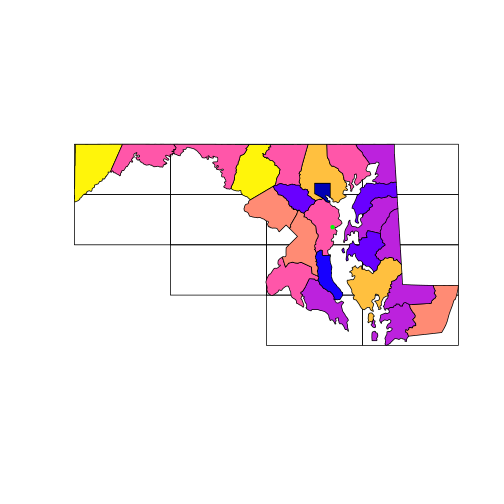
The following code plots the grid first, then the ALAND (land area) column of counties_md.
This plots the county boundaries with the fill color of the polygons corresponding to the
area of the polygon.
The default color scheme means that larger counties appear yellow. Finally, we
overlay the point location of SESYNC.
plot(grid_md)
plot(counties_md['ALAND'],
     add = TRUE)
plot(sesync, col = "green",
     pch = 20, add = TRUE)
But note that the plot function won’t prevent you from layering up geometries
with different coordinate systems: you must safeguard your own plots from this
mistake. The arguments col and pch, by the way, are graphical parameters
used in base R, see ?par.
Spatial Subsetting
An object created with st_read is a data.frame, which is why the dplyr
function filter used above on the non-geospatial column named “STATEFP”
worked normally. The equivalent of a filtering operation on the “geometry”
column is called a spatial “overlay”.
> st_within(sesync, counties_md)
Sparse geometry binary predicate list of length 1, where the predicate was `within'
 1: 5
It can be seen as a type of subsetting based on spatial (rather than numeric or
string) matching. Matching is implemented with functions like st_within(x, y).
The output implies that the 1st (and only) point in sesync is within the 5th
element of counties_md.
The overlay functions in the sf package follow the pattern
st_predicate(x, y) and perform the test “x [is] predicate y”. Some key
examples are:
| st_intersects | boundary or interior of x intersects boundary or interior of y |
| st_within | interior and boundary of x do not intersect exterior of y |
| st_contains | y is within x |
| st_overlaps | interior of x intersects interior of y |
| st_equals | x has the same interior and boundary as y |
Coordinate Transforms
For the next part of this lesson, we import a new polygon layer corresponding to the 1:250k map of US hydrological units (HUC) downloaded from the United States Geological Survey.
shp <- 'data/huc250k'
huc <- st_read(
  shp,
  stringsAsFactors = FALSE)
Compare the coordinate reference systems of counties and huc, as given by
their PROJ.4 strings.
> st_crs(counties_md)$proj4string
[1] "+proj=longlat +datum=NAD83 +no_defs "
> st_crs(huc)$proj4string
[1] "+proj=aea +lat_1=29.5 +lat_2=45.5 +lat_0=23 +lon_0=-96 +x_0=0 +y_0=0 +datum=NAD27 +units=m +no_defs "
The Census data uses unprojected (longitude, latitude) coordinates, but huc is
in an Albers equal-area projection (indicated as "+proj=aea").
The function st_transform() converts an sfc between coordinate reference
systems, specified with the parameter crs = x. A numeric x must be a valid
EPSG code; a character x is interpreted as a PROJ.4 string.
For example, the following character string is a PROJ.4 string which has
a list of parameters that correspond to the EPSG code 42303,
so you could get the same result by typing prj <- 42303.
prj <- '+proj=aea +lat_1=29.5 +lat_2=45.5 \
    +lat_0=23 +lon_0=-96 +x_0=0 +y_0=0    \
    +ellps=GRS80 +towgs84=0,0,0,0,0,0,0   \
    +units=m +no_defs'
PROJ.4 strings contain a reference to the type of projection—this one is another Albers Equal Area—along with numeric parameters associated with that projection. An additional important parameter that may differ between two coordinate systems is the “datum”, which indicates the standard by which the irregular surface of the Earth is approximated by an ellipsoid in the coordinates themselves.
Use st_transform() to assign the two layers and SESYNC’s location
to a common projection string (prj).
This takes a few moments, as it recalculates coordinates for
every vertex in the sfc.
counties_md <- st_transform(
  counties_md,
  crs = prj)
huc <- st_transform(
  huc,
  crs = prj)
sesync <- st_transform(
  sesync,
  crs = prj)
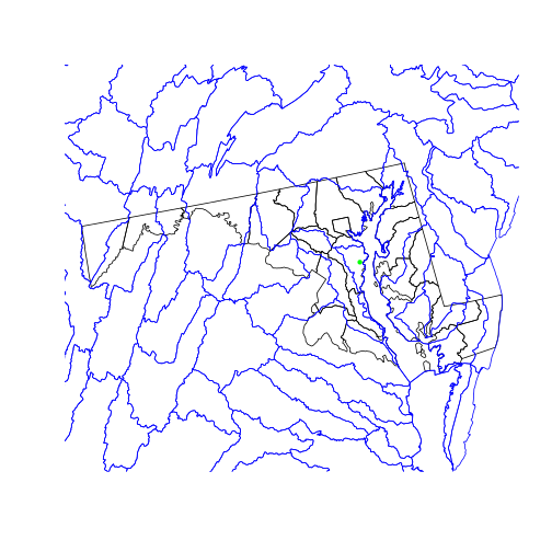
Now that the three objects share a projection, we can plot the county boundaries, watershed boundaries, and SESYNC’s location on a single map.
plot(counties_md$geometry)
plot(huc$geometry,
     border = 'blue', add = TRUE)
plot(sesync, col = 'green',
     pch = 20, add = TRUE)
Geometric Operations
The data for a map of watershed boundaries within the state of MD is all here:
in the country-wide huc and in the state boundary “surrounding” all of
counties_md. To get just the HUCs inside Maryland’s borders:
- remove the internal county boundaries within the state
- clip the hydrological areas to their intersection with the state
The first step is a spatial union operation: we want the resulting object to
combine the area covered by all the multipolygons in counties_md.
state_md <- st_union(counties_md)
plot(state_md)

To perform a union of all sub-geometries in a single sfc, we use the
st_union() function with a single argument. The output, state_md, is a new
sfc that is no longer a column of a data frame. Tabular data can’t safely
survive a spatial union because the polygons corresponding to the attributes
in the table have been combined into a single larger polygon. So the data frame
columns are discarded.
The second step is a spatial intersection, since we want to limit the
polygons to areas covered by both huc and state_md.
huc_md <- st_intersection(
  huc,
  state_md)
Warning: attribute variables are assumed to be spatially constant throughout all
geometries
plot(state_md)
plot(huc_md, border = 'blue',
     col = NA, add = TRUE)
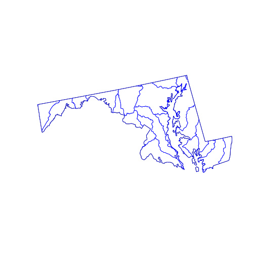
The st_intersection() function intersects its first argument with the second.
The individual hydrological units are preserved but any part of them (or any
whole polygon) lying outside the state_md polygon is cut from the output. The
attribute data remains in the corresponding records of the data.frame, but (as
warned) has not been updated. For example, the “AREA” attribute of any clipped
HUC does not reflect the new polygon.
The GEOS library provides many functions dealing with distances and areas. Many of these are accessible through the sf package, including:
st_buffer: to create a buffer of specific width around a geometryst_distance: to calculate the shortest distance between geometriesst_area: to calculate the area of polygons
Keep in mind that all these functions use planar geometry equations and thus become less precise over larger distances, where the Earth’s curvature is noticeable. To calculate geodesic distances that account for that curvature, check out the geosphere package.
Raster Data
Raster data is a matrix or cube with additional spatial metadata (e.g. extent,
resolution, and projection) that allows its values to be mapped onto geographical
space. The raster package provides the eponymous raster() function
for reading the many formats of such data.
The National Land Cover Database is a 30m resolution grid of cells classified as forest, crops, wetland, developed, etc., across the continental United States. The file provided in this lesson is cropped and reduced to a lower resolution in order to speed processing.
library(raster)
nlcd <- raster("data/nlcd_agg.grd")
By default, raster data is not loaded into working memory, as you can confirm
by checking the R object size with object.size(nlcd). This means that unlike
most analyses in R, you can actually process raster datasets larger than the RAM
available on your computer; the raster package automatically loads pieces of the
data and computes on each of them in sequence.
The default print method for a raster object is a summary of metadata contained
in the raster file.
> nlcd
class      : RasterLayer
dimensions : 2514, 3004, 7552056  (nrow, ncol, ncell)
resolution : 150, 150  (x, y)
extent     : 1394535, 1845135, 1724415, 2101515  (xmin, xmax, ymin, ymax)
crs        : +proj=aea +lat_1=29.5 +lat_2=45.5 +lat_0=23 +lon_0=-96 +x_0=0 +y_0=0 +ellps=GRS80 +towgs84=0,0,0,0,0,0,0 +units=m +no_defs
source     : /nfs/public-data/training/nlcd_agg.grd
names      : nlcd_2011_landcover_2011_edition_2014_03_31
values     : 0, 95  (min, max)
attributes :
        ID      COUNT Red Green Blue Land.Cover.Class Opacity
 from:   0 7854240512   0     0    0     Unclassified       1
  to : 255          0   0     0    0                        0
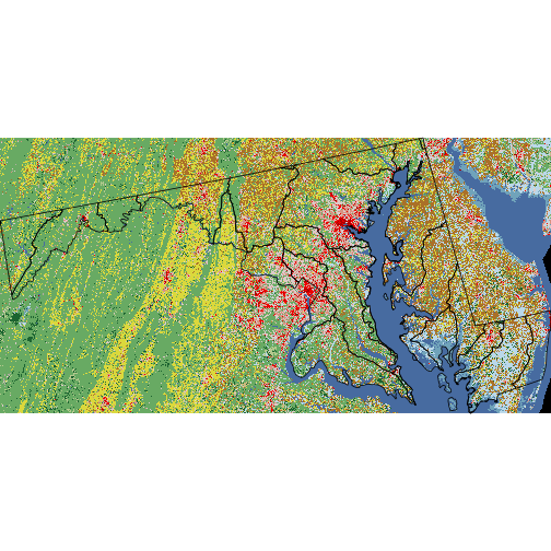
The plot method interprets the pixel values of the raster matrix according to a
pre-defined color scheme.
> plot(nlcd)
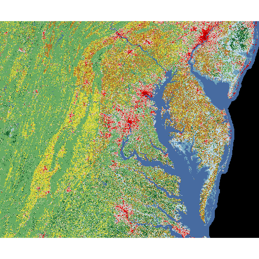
The crop() function trims a raster object to a given spatial “extent” (or
range of x and y values).
Here, we convert the nlcd raster’s bounding box to a 2x2 matrix of the lower left
and upper right corners, then crop the raster
to the extent of the huc_md polygon, then display both layers on the same map.
(We can plot polygon and raster layers together on the same map, just like we can plot
multiple polygon layers—as long as they have the same coordinate reference system!)
Also note that the transformed raster is now loaded in R memory, as indicated by
the size of nlcd. We could have also saved the output to disk by specifying an
optional filename argument to crop; the same is true for many other
functions in the raster package.
extent <- matrix(st_bbox(huc_md), nrow=2)
nlcd <- crop(nlcd, extent)
plot(nlcd)
plot(huc_md, col = NA, add = TRUE)
A raster is fundamentally a data matrix, and individual pixel values can be extracted by regular matrix subscripting. For example, the value of the bottom-left corner pixel:
> nlcd[1, 1]
[1] 41
The meaning of this number is not immediately clear. For this particular dataset, the mapping of values to land cover classes is described in the data attributes:
> head(nlcd@data@attributes[[1]])
  ID      COUNT Red     Green Blue Land.Cover.Class Opacity
1  0 7854240512   0 0.0000000    0     Unclassified       1
2  1          0   0 0.9764706    0                        1
3  2          0   0 0.0000000    0                        1
4  3          0   0 0.0000000    0                        1
5  4          0   0 0.0000000    0                        1
6  5          0   0 0.0000000    0                        1
Notice the @ syntax for extracting the attributes from the nlcd raster object.
The @ operator is used to access properties of an object known as “slots.” These
slots are nested, so we have to access the slot named data from the RasterLayer
object, which itself has a slot called attributes, which is a list with the attribute
table as its first element(!)
The Land.Cover.Class vector gives string names for the land cover type
corresponding to the matrix values. Note that we need to add 1 to the raster
value, since these go from 0 to 255, whereas the indexing in R begins at 1.
nlcd_attr <- nlcd@data@attributes
lc_types <- nlcd_attr[[1]]$Land.Cover.Class
> levels(lc_types)
 [1] ""                              "Barren Land"
 [3] "Cultivated Crops"              "Deciduous Forest"
 [5] "Developed, High Intensity"     "Developed, Low Intensity"
 [7] "Developed, Medium Intensity"   "Developed, Open Space"
 [9] "Emergent Herbaceuous Wetlands" "Evergreen Forest"
[11] "Hay/Pasture"                   "Herbaceuous"
[13] "Mixed Forest"                  "Open Water"
[15] "Perennial Snow/Ice"            "Shrub/Scrub"
[17] "Unclassified"                  "Woody Wetlands"
Raster Math
Mathematical functions called on a raster get applied to each pixel. For a
single raster r, the function log(r) returns a new raster where each pixel’s
value is the log of the corresponding pixel in r.
Likewise, addition with r1 + r2 creates a raster where each pixel is the sum of the
values from r1 and r2, and so on. Naturally, spatial attributes of rasters
(e.g. extent, resolution, and projection) must match for functions that operate
pixel-wise on multiple rasters.
Logical operations work too: r1 > 5 returns a raster with pixel values TRUE
or FALSE and is often used in combination with the mask() function.
pasture <- mask(nlcd, nlcd == 81,
    maskvalue = FALSE)
plot(pasture)
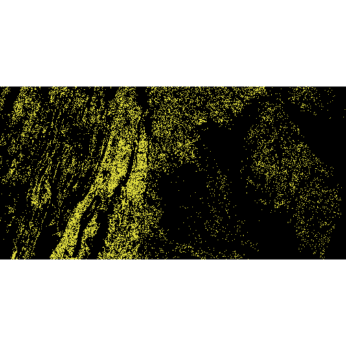
We use the mask function with the logical condition nlcd == 81 and specify that we want to
unset pixel values where the mask is false (maskvalue = FALSE). This results in a raster
where all pixels that are not classified as pasture (code 81) are removed.
To further reduce the resolution of the nlcd raster, the aggregate()
function combines values in a block of a given size using a given function.
nlcd_agg <- aggregate(nlcd,
    fact = 25, fun = modal)
nlcd_agg@legend <- nlcd@legend
plot(nlcd_agg)
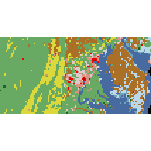
Here, fact = 25 means that we are aggregating blocks 25 x 25 pixels and fun =
modal indicates that the aggregate value is the mode of the original pixels
(averaging would not work since land cover is a categorical variable).
Crossing Rasters with Vectors
Raster and vector geospatial data in R require different packages. The creation of geospatial tools in R has been a community effort, and not necessarily a well-organized one. Development is still ongoing on many packages dealing with raster and vector data. One current stumbling block is that the raster package, which is tightly integrated with the older sp package, has not fully caught up to the sf package. The stars package aims to remedy this problem, and others, but has not yet released a “version 1.0” (it’s at 0.4 as of this writing). In addition, the terra package, which is better integrated with sf, may ultimately replace the raster package. It is also still in development (version 0.6 as of this writing).
Although not needed in this lesson, you may notice in some cases that it is necessary to
convert a vector object from sf (class beginning with sfc*) to sp
(class beginning with Spatial*) for the vector object to interact with rasters.
You can do this by calling sp_object <- as(sf_object, 'Spatial').
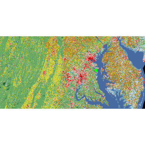
The extract function allows subsetting and aggregation of raster values based
on a vector spatial object. For example we might want to extract the NLCD land cover
class at SESYNC’s location.
plot(nlcd)
plot(sesync, col = 'green',
     pch = 16, cex = 2, add = TRUE)
Pull the coordinates from the sfc object containing SESYNC’s point location and call extract.
When extracting by point locations, the result is a vector of values corresponding to each point.
sesync_lc <- extract(nlcd, st_coordinates(sesync))
> lc_types[sesync_lc + 1]
[1] Developed, Medium Intensity
18 Levels:  Barren Land Cultivated Crops ... Woody Wetlands
When extracting with a polygon, the output is a vector of all raster values for pixels falling within that polygon. This code extracts all pixels within the first polygon in the Maryland county data frame.
county_nlcd <- extract(nlcd_agg,
    counties_md[1,])
> table(county_nlcd)
county_nlcd
11 21 22 23 24 41
 3  1  4  5  2  1
To get a summary of raster values for each polygon in an sfc
object, add an aggregation function to extract via the fun argument. For
example, fun = modal gives the most common land cover type for each polygon in
huc_md.
modal_lc <- extract(nlcd_agg,
    huc_md, fun = modal)
huc_md <- huc_md %>%
  mutate(modal_lc = lc_types[modal_lc + 1])
> huc_md
Simple feature collection with 30 features and 11 fields
geometry type:  GEOMETRY
dimension:      XY
bbox:           xmin: 1396621 ymin: 1837626 xmax: 1797029 ymax: 2037741
CRS:            +proj=aea +lat_1=29.5 +lat_2=45.5
    +lat_0=23 +lon_0=-96 +x_0=0 +y_0=0
    +ellps=GRS80 +towgs84=0,0,0,0,0,0,0
    +units=m +no_defs
First 10 features:
         AREA PERIMETER HUC250K_ HUC250K_ID HUC_CODE              HUC_NAME REG
1  6413577966  454290.2      904        916 02050306     Lower Susquehanna  02
2  1982478663  292729.7      916        927 02040205  Brandywine-Christina  02
3  5910074657  503796.5      938        948 02070004 Conococheague-Opequon  02
4  3159193443  506765.4      957        968 02060002     Chester-Sassafras  02
5  4580816836  433034.1      967        978 05020006          Youghiogheny  05
6  2502118608  252945.8      976        987 02070009              Monocacy  02
7  3483549988  415851.4      988        999 02060003    Gunpowder-Patapsco  02
8  3582821909  935625.3      993       1004 02060001  Upper Chesapeake Bay  02
9  3117956776  378807.0      999       1009 02070003          Cacapon-Town  02
10 3481485179  373451.5     1003       1013 02070002  North Branch Potomac  02
    SUB    ACC      CAT                       geometry         modal_lc
1  0205 020503 02050306 MULTIPOLYGON (((1683575 203... Deciduous Forest
2  0204 020402 02040205 MULTIPOLYGON (((1707075 202...      Hay/Pasture
3  0207 020700 02070004 POLYGON ((1563403 2008455, ...      Hay/Pasture
4  0206 020600 02060002 POLYGON ((1701439 2037188, ... Cultivated Crops
5  0502 050200 05020006 POLYGON ((1441528 1985664, ... Deciduous Forest
6  0207 020700 02070009 POLYGON ((1610557 2016043, ... Cultivated Crops
7  0206 020600 02060003 POLYGON ((1610557 2016043, ... Deciduous Forest
8  0206 020600 02060001 MULTIPOLYGON (((1691021 201...       Open Water
9  0207 020700 02070003 POLYGON ((1496410 1995810, ... Deciduous Forest
10 0207 020700 02070002 POLYGON ((1468299 1990565, ... Deciduous Forest
Interactive Maps
The leaflet package is an R interface to the leaflet JavaScript library. It produces interactive maps (with controls to zoom, pan and toggle layers) combining local data with base layers from web mapping services.
The leaflet() function creates an empty leaflet map to which layers can be
added using the pipe (%>%) operator. The addTiles functions adds a base
tiled map; by default, it imports tiles from OpenStreetMap. We center and zoom
the map with setView.
library(leaflet)
leaflet() %>%
    addTiles() %>%
    setView(lng = -77, lat = 39,
        zoom = 7)
The map shows up in the “Viewer” tab in RStudio because, like everything with JavaScript, it relies on your browser to render the image.
Spatial datasets (points, lines, polygons, rasters) in your R environment can also be added as map layers, provided they are in lat/lon coordinates (EPSG:4326). Leaflet will try to make the necessary transformation to display your data in EPSG:3857.
leaflet() %>%
    addTiles() %>%
    addPolygons(
        data = st_transform(huc_md, 4326)) %>%
    setView(lng = -77, lat = 39,
        zoom = 7)
Leaflet can access open data from various web mapping services (WMS), including real-time weather radar data from the Iowa Environmental Mesonet.
leaflet() %>%
    addTiles() %>%
    addWMSTiles(
        "http://mesonet.agron.iastate.edu/cgi-bin/wms/nexrad/n0r.cgi",
        layers = "nexrad-n0r-900913", group = "base_reflect",
        options = WMSTileOptions(format = "image/png", transparent = TRUE),
        attribution = "Weather data © 2012 IEM Nexrad") %>%
    setView(lng = -77, lat = 39,
        zoom = 7)
Use the map controls to zoom away from the current location and find ongoing storm events.
This lesson only provides a very brief introduction to leaflet. For a more in-depth tutorial, check out the SESYNC lesson on leaflet in R.
Resources
- raster package vignette.
- R.S. Bivand, E.J. Pebesma and V. Gómez-Rubio (2013) Applied Spatial Data Analysis with R. UseR! Series, Springer.
- R. Lovelace et al., Geocomputation with R
- F. Rodriguez-Sanchez. Spatial data in R: Using R as a GIS.
- CRAN Task View: Analysis of Spatial Data
- P. Marchand. Introduction to geospatial data analysis in R uses the
starspackage
More packages to try out
- exactextractr: quickly summarizes rasters across polygons
- rasterVis: supplements the raster package for improved visualizations
- velox: fast raster extraction still in development on GitHub
Exercises
Exercise 1
Produce a map of Maryland counties with the county that contains SESYNC colored in red.
Exercise 2
Use st_buffer to create a 5km buffer around the state_md border and plot it as a dotted line (plot(..., lty = 'dotted')) over the true state border. Hint: check the layer’s units with st_crs() and express any distance in those units.
Exercise 3
The function cellStats aggregates across an entire raster. Use it to figure out the proportion of nlcd pixels that are covered by deciduous forest (value = 41).
Solutions
Solution 1
> plot(counties_md$geometry)
> overlay	<- st_within(sesync, counties_md)
> counties_sesync <- counties_md[overlay[[1]], 'geometry']
> plot(counties_sesync, col = "red", add = TRUE)
> plot(sesync, col = 'green', pch = 20, add = TRUE)
Solution 2
> bubble_md <- st_buffer(state_md, 5000)
> plot(state_md)
> plot(bubble_md, lty = 'dotted', add = TRUE)
Solution 3
> cellStats(nlcd == 41, "mean")
If you need to catch-up before a section of code will work, just squish it's 🍅 to copy code above it into your clipboard. Then paste into your interpreter's console, run, and you'll be ready to start in on that section. Code copied by both 🍅 and 📋 will also appear below, where you can edit first, and then copy, paste, and run again.
# Nothing here yet!