Intersections, Zonal Statistics, and Distance

####################################   Suitability Analysis   #######################################
############################  Selection of parcels for conservation   #######################################
# This script performs basic analyses for the Exercise 3 of the AGG and SESYNC Geospatial Analysis course.
# We are using data from the state of Florida.The overall goal is to perform a analysis with 
# multi-criteria/sustainabiltiy analysis to select areas suitable 
# for conservation.     
#
#Goal: Determine the ten (10) parcels of land within Clay County in the focus zone most suitable for purchase
#towards conversion to land conservation.
#
#AUTHORS: Benoit Parmentier                                             
#DATE CREATED: 03/17/2017 
#DATE MODIFIED: 03/25/2019
#Version: 2
#PROJECT: SESYNC and AAG 2019 workshop/Short Course preparation
#TO DO:
#
#COMMIT: general modif and adding sf
#
#################################################################################################

###Loading R library and packages                                                      

library(sp) # spatial/geographfic objects and functions
library(rgdal) #GDAL/OGR binding for R with functionalities
library(spdep) #spatial analyses operations, functions etc.
library(gtools) # contains mixsort and other useful functions
library(maptools) # tools to manipulate spatial data
library(parallel) # parallel computation, part of base package no
library(rasterVis) # raster visualization operations
library(raster) # raster functionalities
library(forecast) #ARIMA forecasting
library(xts) #extension for time series object and analyses
library(zoo) # time series object and analysis
library(lubridate) # dates functionality
library(colorRamps) #contains matlab.like color palette
library(rgeos) #contains topological operations
library(sphet) #contains spreg, spatial regression modeling
library(BMS) #contains hex2bin and bin2hex, Bayesian methods
library(bitops) # function for bitwise operations
library(foreign) # import datasets from SAS, spss, stata and other sources
library(gdata) #read xls, dbf etc., not recently updated but useful
library(classInt) #methods to generate class limits
library(plyr) #data wrangling: various operations for splitting, combining data
#library(gstat) #spatial interpolation and kriging methods
library(readxl) #functionalities to read in excel type data
library(sf)

###### Functions used in this script

#function_preprocessing_and_analyses <- "fire_alaska_analyses_preprocessing_functions_03102017.R" #PARAM 1
#script_path <- "/home/attendee/data/AAG2017_spatial_temporal_analysis_R/R_scripts"
#source(file.path(script_path,function_preprocessing_and_analyses)) #source all functions used in this script 1.
create_dir_fun <- function(outDir,out_suffix=NULL){
  #if out_suffix is not null then append out_suffix string
  if(!is.null(out_suffix)){
    out_name <- paste("output_",out_suffix,sep="")
    outDir <- file.path(outDir,out_name)
  }
  #create if does not exists
  if(!file.exists(outDir)){
    dir.create(outDir)
  }
  return(outDir)
}

#####  Parameters and argument set up ###########

in_dir_var <- "data"
out_dir <- "."

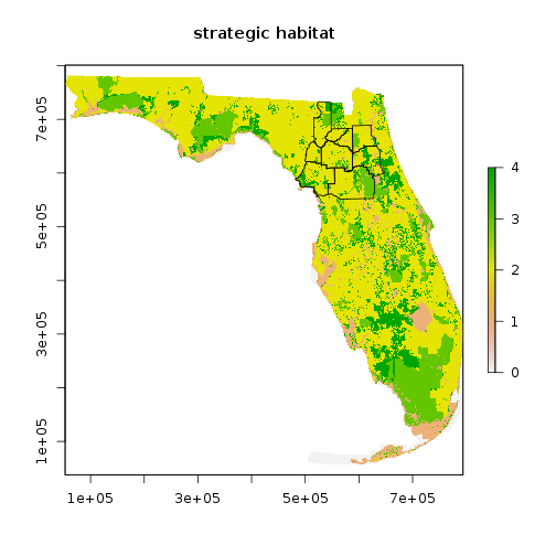
strat_hab_fname <- "Strat_hab_con_areas1/Strat_hab_con_areas1.tif" #1)Strategic Habitat conservation areas raster file
regional_counties_fname <- "Regional_Counties" #2) County shapefile
roads_fname <- "roads_counts/roads_counts.tif" #3) Roads count raster
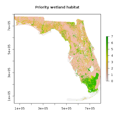
priority_wet_habitats_fname <- "Priority_Wet_Habitats1/Priority_Wet_Habitats1.tif" #4) Priority Wetlands Habitat raster file
clay_parcels_fname <- "Clay_Parcels" #5) Clay County parcel shapefile
habitat_fname <- "Habitat/Habitat.tif" #6) General Habitat raster file
biodiversity_hotspot_fname <- "Biodiversity_Hot_Spots1/Biodiversity_Hot_Spots1.tif" #7) Biodiversity hotspot raster file
florida_managed_areas_fname <- "flma_jun13" #8) Florida managed areas shapefile
focus_zone1_filename <- "focus_zone1/focus_zone1.tif" #9) focus zone as raster file

##Additional data: 
#roads_distance_exercise3.tif: distance to roads
#r_flma_clay_bool_distance_exercise3.tif: distance to Florida Mangement Areas

gdal_installed <- TRUE #if true use the system/shell command else use the distance layer provided
file_format <- ".tif" #PARAM5
NA_flag_val <- -9999 #PARAM7
out_suffix <-"exercise3_03212019" #output suffix for the files and ouptu folder #PARAM 8
create_out_dir_param=TRUE #PARAM9

################# START SCRIPT ###############################

## First create an output directory

if(is.null(out_dir)){
  out_dir <- dirname(in_dir_var) #output will be created in the input dir
}

out_suffix_s <- out_suffix #can modify name of output suffix
if(create_out_dir_param==TRUE){
  out_dir <- create_dir_fun(out_dir,out_suffix_s)
}

####  PART I: EXPLORE DATA READ AND DISPLAY INPUTS #######

##Inputs:
#1) Strategic Habitat conservation areas raster file
#2) County shapefile
#3) Roads shapefile
#4) Priority Wetlands Habitat raster file
#5) Clay County parcel shapefile
#6) General Habitat raster file
#7) Biodiversity hotspot raster file
#8) Florida managed areas shapefile
#9) Focus area as raster file

## Read in the datasets
r_strat_hab <- raster(file.path(in_dir_var,strat_hab_fname))
reg_counties_sf <- st_read(file.path(in_dir_var,regional_counties_fname)) 

r_roads <- raster(file.path(in_dir_var,roads_fname))
r_priority_wet_hab <- raster(file.path(in_dir_var,priority_wet_habitats_fname))

clay_sf <- st_read(file.path(in_dir_var,clay_parcels_fname)) #large file

r_habitat <- raster(file.path(in_dir_var,habitat_fname))
r_bio_hotspot <- raster(file.path(in_dir_var,biodiversity_hotspot_fname))

flma_sf <- st_read(file.path(in_dir_var,florida_managed_areas_fname)) 

r_focus_zone1 <- raster(file.path(in_dir_var,focus_zone1_filename))

## Visualize a few datasets
plot(r_strat_hab, main="strategic habitat")
plot(reg_counties_sf$geometry,add=T)

plot(r_priority_wet_hab, main="Priority wetland habitat")

#plot(r_habitat,add=T)

##### Before starting the production of the sustainability factor let's check the projection, 
#resolution for each layer relevant to the calculation

#raster layers:

list_raster <- c(r_strat_hab,r_priority_wet_hab,r_habitat,r_bio_hotspot)

## Examine information on rasters using lapply
lapply(list_raster,function(x){res(x)}) #spatial resolution

lapply(list_raster,function(x){projection(x)}) #spatial projection

lapply(list_raster,function(x){extent(x)}) #extent of rasters

### PART 0: generate reference layer

## Let's use the resolution 55x55 m as the reference since it corresponds to finer resolution relevant
# for this study. The focus region provides the extent for the final step.
## Select clay county
clay_county_sf <- subset(reg_counties_sf,NAME=="CLAY")

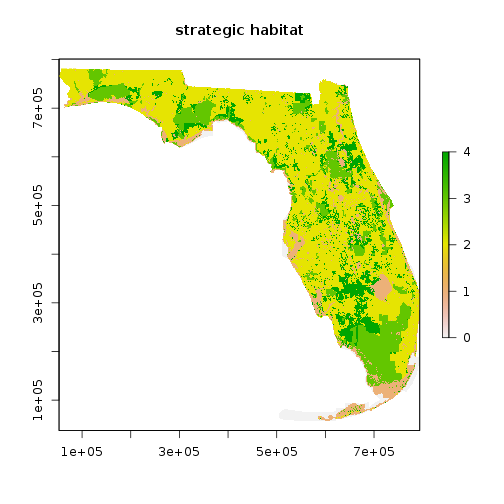
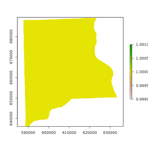
plot(r_strat_hab, main="strategic habitat")

## Crop r_strat_hab
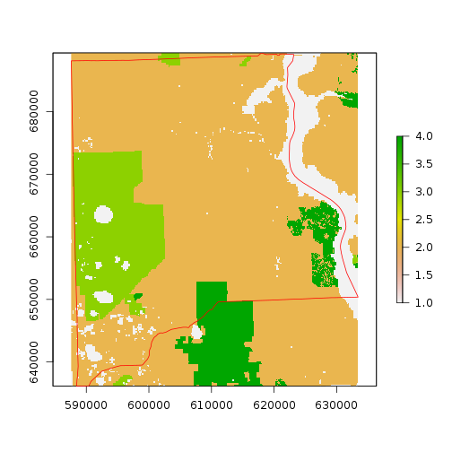
r_ref <- crop(r_strat_hab,as.vector(st_bbox(clay_county_sf))[c(1, 3, 2, 4)]) #make a reference image for use in the processing

plot(r_ref)
plot(clay_county_sf$geometry,border="red",add=T)

r_clay <- rasterize(clay_county_sf,r_ref) #this can be used as mask for the study area
freq(r_clay) #check the distribution of values: 1 and NA 

##Use raster of Clay county definining the study area to mask pixels
plot(r_clay)

dim(r_clay) #number of rows and columns as well as number of layers/bands

####  PART II :  HIGH BIODIVERSITY SUITABILITY LAYERS #######
## IDENTIFY LANDS WITH HIGH NATIVE BIODIVERSITY

### STEP 1: Strategic Habitat conservation areas

#Input data layer: Habitat
#We will use information from the National Heritage Froundation to reclassify the Habitat layer as input
#criterion for the suitability analysis.
#Criteria for value assignment: Habitat ranked by the Natural Heritage Program as having high native
#biodiversity were given a value of 9. Habitat ranked as having a moderate native biodiversity were given
#a value of 5, and all other habitat types were given a value of 1.
#Rationale for value assignment: Certain habitat types are known to have higher native biodiversity than
#others, consequently those with higher native biodiversity were given higher suitability rankings.
#Output: Habitat Biodiversity 

#strategic habitat conservation areas
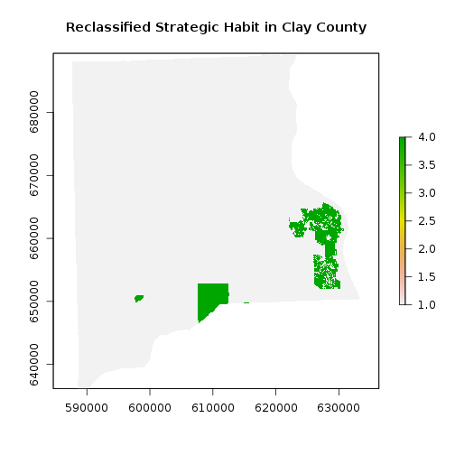
r_strat_hab_w <- crop(r_strat_hab,r_clay) #Crop habitat conservation layer covering the State of Florida
r_strat_hab_masked <- mask(r_strat_hab_w,r_clay) # Mask layer matching the Clay county area

## Now reclassify: create a matrix of reclassification
#values are: from, to, assigned value
m <- c(5, 1000, 9,   #use 1000 as upper limit, can be any value greater than max
       4, 5, 5,  
       1, 3, 1)  

rclmat <- matrix(m, ncol=3, byrow=TRUE)

#?raster::reclassify: to find out information on the function

rc_strat_hab_reg <- reclassify(r_strat_hab_masked, rclmat)
plot(rc_strat_hab_reg,main="Reclassified Strategic Habit in Clay County")

### STEP 2: Identify Lands With High Native Biodiversity based on species count 

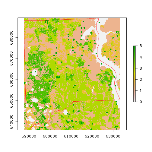
## Crop bio raster
r_bio_hotspot_w <- crop(r_bio_hotspot,as.vector(st_bbox(clay_county_sf))[c(1, 3, 2, 4)])
plot(r_bio_hotspot_w)
plot(clay_county_sf$geometry,border="red",add=T)

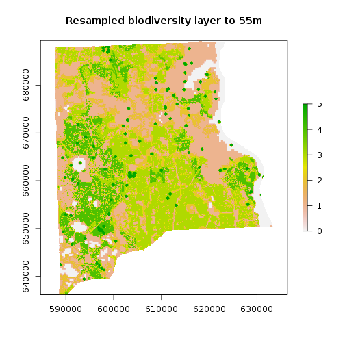
#match resolution:
projection(r_bio_hotspot_w)==projection(r_clay) #projection match

res(r_bio_hotspot_w)==res(r_clay) #the resolutions do not match, we will need to resample

## Find about resample
#?raster::resample #to find out about the resample function from the raster package
r_bio_hotspot_reg <- raster::resample(x=r_bio_hotspot_w,y=r_clay, method="bilinear") #Use resample to match resolutions
r_bio_hotspot_reg <- mask(r_bio_hotspot_reg,r_clay) ## It now works because resolutions were matched
plot(r_bio_hotspot_reg,main="Resampled biodiversity layer to 55m")

### Reclassify using instructions/information given to us:

m <- c(9, 1000, 9,  
       5, 8, 8,  
       3, 4, 7,  
       1, 2,1)
rclmat <- matrix(m, ncol=3, byrow=TRUE)

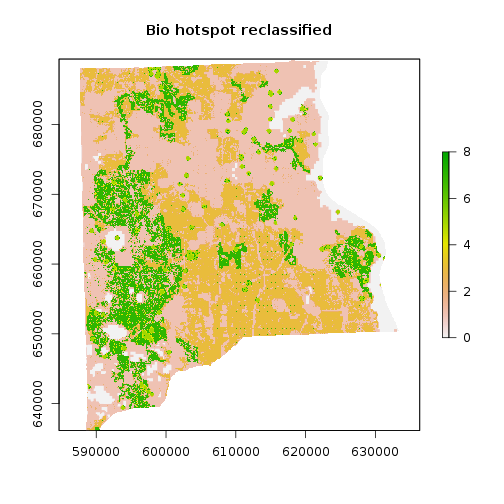
rc_bio_hotspot_reg <- reclassify(r_bio_hotspot_reg, rclmat)

plot(rc_bio_hotspot_reg, main="Bio hotspot reclassified")

### STEP 3: Wetland priority 

#Input data layer: Priority Wetland Habitats
#Criteria for value assignment: Values were assigned based on the number of focal species present in
#each cell. The value of 9 was assigned to 10–12 wetland focal species, 8 was assigned to 7–9 wetland focal
#species, 7 was assigned to 4–6 wetland focal species and 4–6 upland focal species, 6 was assigned to
#1–3 wetland or upland focal species. The value 1 was assigned to all other cells.
#Rationale for value assignment: The better the habitat for focal wetland species, the higher the priority.
#Output: Wetland Biodiversity 

#check projection
projection(r_priority_wet_hab)

## Crop Wetland priority raster
r_priority_wet_hab_w <- crop(r_priority_wet_hab,as.vector(st_bbox(clay_county_sf))[c(1, 3, 2, 4)])

#match resolution:
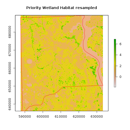
r_priority_wet_hab_reg <- raster::resample(r_priority_wet_hab_w,r_clay, method='bilinear') #resolution matching the study region

#r_priority_wet_hab_reg <- mask(r_priority_wet_hab_reg,r_clay) ## Does not work!! because resolution doesn't match
plot(r_priority_wet_hab_reg,main="Priority Wetland Habitat resampled")
plot(clay_county_sf$geometry,border="red",add=T)

### Now reclass
#The value of 9 was assigned to 10–12 wetland focal species, 8 was assigned to 7–9 wetland focal
#species, 7 was assigned to 4–6 wetland focal species and 4–6 upland focal species, 6 was assigned to
#1–3 wetland or upland focal species. The value 1 was assigned to all other cells.

m <- c(10, 12, 9,  
       7, 9, 8,  
       4, 6, 7,  
       1, 3,6,
       -1, 1,1)

rclmat <- matrix(m, ncol=3, byrow=TRUE)

rc_priority_wet_hab_reg <- reclassify(r_priority_wet_hab_reg, rclmat)
freq_tb <- freq(rc_priority_wet_hab_reg)
freq_tb

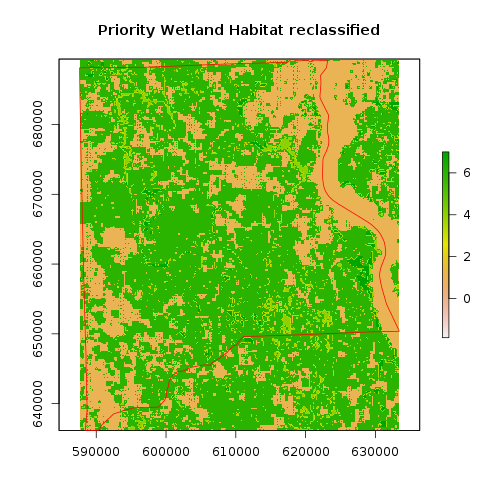
plot(rc_priority_wet_hab_reg,main="Priority Wetland Habitat reclassified")
plot(clay_county_sf$geometry,border="red",add=T)

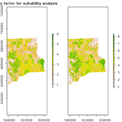
### STEP 4: Combine all the three input criteria layers with weigthed/unweighted sum

f_weights <- c(1,1,1)/3
r_bio_es_factor <- (f_weights[1]*rc_strat_hab_reg + f_weights[2]*rc_bio_hotspot_reg + f_weights[3]*rc_priority_wet_hab_reg) #weighted sum

f_weights <- c(1,1.5,1.5)/3
r_bio_ws_factor <- (f_weights[1]*rc_strat_hab_reg + f_weights[2]*rc_bio_hotspot_reg + f_weights[3]*rc_priority_wet_hab_reg) #weighted sum

r_bio_factor <- stack(r_bio_es_factor,r_bio_ws_factor)
names(r_bio_factor) <- c("equal_weights","weigthed_sum")
plot(r_bio_factor,main="Bio factor for suitability analysis")

out_suffix_str <- paste0(names(r_bio_factor),"_",out_suffix) # this needs to be matching the number of outputs files writeRaste

##Write out raster file:
writeRaster(r_bio_factor,filename=file.path(out_dir,"r_bio_factor_clay.tif"),
            bylayer=T,datatype="FLT4S",options="COMPRESS=LZW",suffix=out_suffix_str,overwrite=T)

####  PART III : SUITABILITY LAYERS #######

#IDENTIFY POTENTIAL CONSERVATION LANDS IN RELATION WITH DISTANCE TO ROADS AND EXISTING MANAGED LANDS
#GOAL: Create two raster maps showing lands in Clay County, 
#Florida that have would have higher conservation potential based on 
#local road density and distance from existing managed lands using a combination 
#of the Clip, Extract by Mask, Euclidean Distance, Line Density, Project, Reclassify, and Weighted Sum tools.

#Step 1: prepare files to create a distance to road layer

### Processs roads first
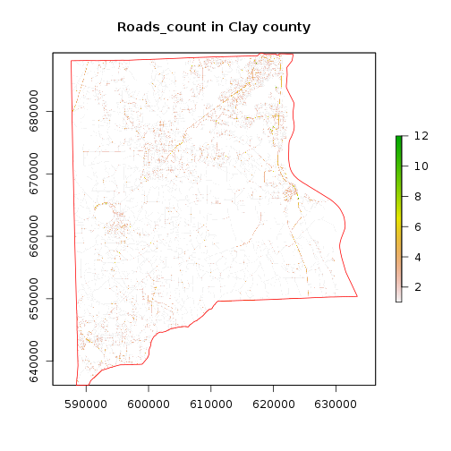
plot(r_roads,main="Roads_count in Clay county")
r_roads_bool <- r_roads > 0
plot(clay_county_sf$geometry,border="red",add=T)

NAvalue(r_roads_bool ) <- 0 
roads_bool_fname <- file.path(out_dir,paste0("roads_bool_",out_suffix,file_format))
r_roads_bool <- writeRaster(r_roads_bool,filename=roads_bool_fname,overwrite=T)

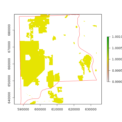
#setp 2: prepare files to create a distance to existing managed land

r_flma_clay <- rasterize(flma_sf,r_clay,"OBJECTID_1",fun="max")

r_flma_clay_bool <- r_flma_clay > 0
NAvalue(r_flma_clay_bool) <- 0
r_flma_clay_bool_fname <- file.path(out_dir,paste0("r_flma_clay_bool_",out_suffix,file_format))
r_flma_clay_bool <- writeRaster(r_flma_clay_bool,filename=r_flma_clay_bool_fname,overwrite=T)
plot(r_flma_clay_bool,"Management areas in Clay County")
plot(clay_county_sf$geometry,border="red",add=T)

if(gdal_installed==TRUE){
  
  ## Roads
  srcfile <- roads_bool_fname
  dstfile_roads <- file.path(out_dir,paste("roads_distance_",out_suffix,file_format,sep=""))
  n_values <- "1"
  
  ### Note that gdal_proximity doesn't like when path is too long
  cmd_roads_str <- paste("gdal_proximity.py",srcfile,dstfile_roads,"-values",n_values,sep=" ")
  #cmd_str <- paste("gdal_proximity.py", srcfile, dstfile,sep=" ")
  
  ### Prepare command for FLMA
  
  srcfile <- r_flma_clay_bool_fname 
  dstfile_flma <- file.path(out_dir,paste("r_flma_clay_bool_distance_",out_suffix,file_format,sep=""))
  n_values <- "1"
  
  ### Note that gdal_proximity doesn't like when path is too long
  cmd_flma_str <- paste("gdal_proximity.py",srcfile,dstfile_flma,"-values",n_values,sep=" ")
  #cmd_str <- paste("gdal_proximity.py", srcfile, dstfile,sep=" ")
  
  sys_os <- as.list(Sys.info())$sysname
  
  if(sys_os=="Windows"){
    shell(cmd_roads_str)
    shell(cmd_flma_str)
  }else{
    system(cmd_roads_str)
    system(cmd_flma_str)
  }
  r_flma_distance <- raster(dstfile_flma)
  r_roads_distance <- raster(dstfile_roads)
  
}else{
  r_roads_distance <- raster(file.path(in_dir_var,"additional_data",paste("roads_distance_exercise3",file_format,sep="")))
  r_flma_distance <- raster(file.path(in_dir_var,"additional_data",paste("r_flma_clay_bool_distance_exercise3",file_format,sep="")))
}

#Now rescale the distance...
min_val <- cellStats(r_roads_distance,min) 
max_val <- cellStats(r_roads_distance,max)

#Linear rescaling:
#y = ax + b with b=0
#with 9 being new max and 0 being new min
a = (9 - 0) /(max_val - min_val)
r_roads_dist <- r_roads_distance * a

#Get distance from managed land
#b. Which parts of Clay County contain proximity-to-managed-lands characteristics that would make them more favorable to be used as conservation lands?

min_val <- cellStats(r_flma_distance,min) 
max_val <- cellStats(r_flma_distance,max)
a = (9 - 0) /(max_val - min_val) #linear rescaling factor
r_flma_dist <- r_flma_distance * a

####  PART IV : COMBINE FACTORS AND DETERMINE MOST SUITABLE PARCELS #######
#IDENTIFY POTENTIAL CONSERVATION LANDS IN RELATION TO PARCEL SUITABILITY
#GOAL: Create two raster maps showing parcels in Clay County, Florida that have would 
#have higher conservation potential based on parcel values.
#First, factors must be combin  ed to generate a suitability index.

### Step 1:  Combine distance factors with weights...
f_weights <- c(1,1)/2 #factor weights for distance to roads
r_dist_factor <- f_weights[1]*r_roads_dist + f_weights[2]*r_flma_dist #weighted sum with equal weight

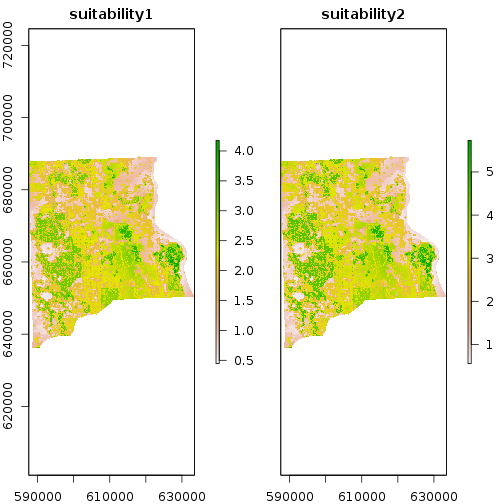
### Step 2: Combine distance factor and bio factor
f_weights <- c(2/3,1/3) #We are weighting factor bio more for this exercise
r_suitability_factor <- f_weights[1]*r_bio_factor + f_weights[2]*r_dist_factor #weighted sum with equal weight
names(r_suitability_factor) <- c("suitability1","suitability2")
plot(r_suitability_factor)

out_suffix_str <- paste0(names(r_suitability_factor),"_",out_suffix) # this needs to be matching the number of outputs files writeRaste

writeRaster(r_suitability_factor,filename=file.path(out_dir,"r_suitability_factor_clay.tif"),
            bylayer=T,datatype="FLT4S",options="COMPRESS=LZW",suffix=out_suffix_str,overwrite=T)

### Step 3: summarize by parcels!!

projection(r_focus_zone1)<- projection(r_clay)

clay_sp_parcels_reg <- st_transform(clay_sf,projection(r_clay))

focus_zone1_sf <- st_as_sfc(st_bbox(r_focus_zone1))

parcels_focus_zone1_sf <- st_intersection(clay_sp_parcels_reg,focus_zone1_sf)

parcels_avg_suitability <- extract(r_suitability_factor,parcels_focus_zone1_sf,fun=mean,sp=T) #takes about 2 minutes, check on docker!!

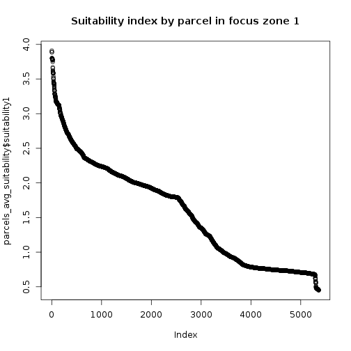
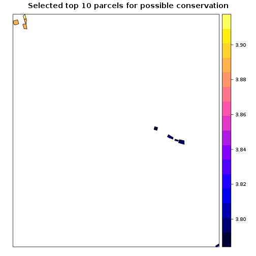
## Select top 10 parcels to target for conservation
parcels_avg_suitability <- parcels_avg_suitability[order(parcels_avg_suitability$suitability1,decreasing = T),] 
plot(parcels_avg_suitability$suitability1,main="Suitability index by parcel in focus zone 1")

spplot(parcels_avg_suitability[1:10,],"suitability1",main="Selected top 10 parcels for possible conservation")

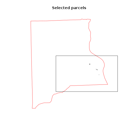
##Figure of selected parcels
plot(clay_county_sf$geometry,border="red",main="Selected parcels")
plot(parcels_avg_suitability[1:10,],add=T)
plot(focus_zone1_sf,add=T)

##############################   END OF SCRIPT    ##########################################