Smart and Interactive Documents
Handouts for this lesson need to be saved on your computer. Download and unzip this material into the directory (a.k.a. folder) where you plan to work.
Lesson Objectives
- Start with “dumb” documents and the basics of Markdown.
- Get “smart” by embedding computed document content.
- Go “interactive” with shiny components.
- Envision an efficient, one-click pipeline with RMarkdown.
Specific Achievements
- Create a slideshow with interactive visualizations.
How Smart?
The reproducible pipeline under construction begins with open data, uses scripts to perform analyses and create visualizations, and ideally ends in a published write-up.
rmarkdown merges code and documentation, allowing you to create automatic reports that include the results of computations and visualizations created on-the-fly.
How Interactive?
Rather than rendering to a static document, RStudio lets you easily inject shiny input and output widgets to documents constructed with RMarkdown. These widgets can accept user input through forms, menus, and sliders, and cause corresponding tables, plots, and other graphical output to dynamically update.
Interactive documents require connection to a live R process, which any user running RStudio can provide, but so can hosting services like www.shinyapps.io.
Markdown
Markdown exists outside of the R environment. Like R, it is both a language and an interpreter.
-
It is a language with special characters and a syntax that convey formatting instructions inside text files.
-
The accompanying interpreter reads text files and outputs one of several types of formatted documents (e.g Word, PDF, and HTML).
RMarkdown
The rmarkdown package bundles the formatting ability of Markdown with the ability to send embedded code to an R interpreter and capture the result.
Seeing is Believing
The lesson’s .Rmd worksheet is an RMarkdown script. Open it and find the
following incantation.
```{r}
x <- rnorm(10)
mean(x)
```
Press the “Knit” button in RStudio to generate the computed document. Note that
after the code we entered is the computed result. As we proceed, fill in each
... in your worksheet, and press the “Knit” button to examine the result.
Markdown Syntax
Before getting to the good stuff, a quick introduction to “dumb” Markdown formatting.
Text and Emphasis
Text in Markdown is rendered as is, albeit in some pre-defined size and font, into an HTML file by default. Text fenced by “*” is translated by the Markdown interpreter into italics for emphasis.
Adding emphasis is an example of “marking up” plain text with a light-weight syntax, i.e. the code is readable before being rendered into a document.
Bulleted Lists
Sequential lines beginning with “-“ are grouped into a bulleted list.
- SQL
- Python
- R
Numbered Lists
Sequential lines beginning with a number are grouped into a numbered list. The actual number you use is irrelevant.
6. SQL
1. Python
5. R
Tables
Separate text with vertical bars (|) to indicate columns of a table and
hyphens (-) to mark the beginning of a table or to separate the header row.
id | treatment
---|----------
1  | control
2  | exclosure
Configuration
Text at the top of a Markdown file and fenced by --- stores configuration.
Variables set here can, for example, change the type of document produced.
---
output: html_document
---
Change the output variable to ioslides_presentation and knit again to generate
output formatted as a slideshow.
---
output: ioslides_presentation
---
Headers
Default formatting for an html_document differs in some cases from an
ioslides_presentation. The use of # to indicate a hierarchy of heading sizes
serves an additional purpose in a slideshow.
# The Biggest Heading

## The Second Biggest Heading

### The Third Biggest Heading
Preformatted Text
Text fenced by either one or three “backticks” (the “`” character) is left untouched by the Markdown interpreter, usually for the purpose of displaying code. Everything else is formatted according to a light-weight syntax.
```
The *emphasis* indicated by asterisks here does not become
italicized, as it would outside a "code fence".
```
That’s three backtick characters, found next to the “1” on QWERTY keyboards, above and below the text. A single backtick leaves code “inline”, while three (or more) backticks indicate a separate block of preformatted text or a “chunk”.
You can write R code in a chunk, but it’s still just “dumb” Markdown.
```
seq(1, 10)
```
R + Markdown
The rmarkdown package evaluates the R expressions within a code fence and
inserts the result into the output document. To send these “code chunks” to the
R interpreter, append {r} to the upper fence.
```{r}
seq(1, 10)
```
Chunk Options
Each code chunk runs under options specified globally or within the {r, ...}
expression. The option echo = FALSE would cause the output to render without
the input. The option eval = FALSE, would prevent evaluation and output
rendering.
```{r, echo = FALSE}
seq(1, 10)
```
Chunk Labels
The first entry after {r will be interpretted as a chunk label if it is not
setting an option. Chunk options are specified after the optional label and
separated by commas. Labels do not show up in the document—we’ll have other
uses for them.
```{r does_not_run, eval = FALSE}
seq(1, 10)
```
Reproducible Pipeline
A pipeline might rely on several scripts that separately aquire data, tidy it, fit or run models, and validate results. Embedding calls to those external scripts is one way to create a one-click pipeline.
Sourced Input
The source function in R includes the contents of a separate file in the
current code chunk. The entire script is evaluated in the current environment.
```{r load_data, echo = FALSE}
source('worksheet.R')
```
The lesson’s .R worksheet is an R script creating a state_movers data frame,
which “sourcing” makes available to following lines as well as subsequent code
chunks.
```{r bar_plot, echo = FALSE}
library(ggplot2)
ggplot(state_movers,
  aes(x = current_state, y = sum_new_movers)) +
  geom_bar(stat = 'identity') +
  theme(axis.text.x = element_text(
    angle = 90, hjust = 1))
```
If your entire pipeline can be scripted in R, you could embed the entire analysis in code chunks within your write-up. The better practice demonstrated here is “modularizing” your analysis by splitting it into isolated scripts, and then using an rmarkdown document to execute the pipeline.
Alternative Engines
RMarkdown code chunks are not limited to R. Several “engines”, including Python and SQL, can be used for code written directly into a code chunk.
```{python}
greeting = 'Hello, {}!'
print(greeting.format('World'))
```
Access to your operating system shell, for example the Linux Bash interpreter, provides a way to run any scripted pipeline step.
```{bash}
echo "Hello, ${USER}!"
```
An important distinction between sourced and non-sourced input is the inabillity
of interpreters other than R to return R objects. By using source, an R script
is run in the current R session, which provides an easy way to pass data between
scripts. Typically, file-based input and output is necessary for multi-lingual
pipelines. For Python, however, the
reticulate
package provides a bi-directional interface.
Efficient Pipelines
There is no reason to run every step of a pipeline after making changes “downstream”. Like more comprehensive software for automating pipelines, rmarkdown includes the notion of tracking dependencies and caching results. Cached code chunks are not re-evaluated unless the content of the code changes.
Enable cache in a setup chunk to turn off re-evaluation of any code
chunk that has not been modified since the last knit.
```{r setup, include = FALSE}
library(knitr)
opts_chunk$set(
  message = FALSE,
  warning = FALSE,
  cache = TRUE)
```
Cache
- Render the worksheet again to create a cache for each code chunk.
- Then modify your
bar_plotchunk to sort the bars and render again.
```{r bar_plot}
library(ggplot2)
ggplot(state_movers,
  aes(
    x = reorder(current_state, -sum_new_movers),
    y = sum_new_movers)) +
  geom_bar(stat = 'identity') +
  theme(axis.text.x = element_text(
    angle = 90, hjust = 1))
```
The “slow” load_data chunk zips right by, using its cache, but the plot will
change because you modified that code chunk.
Cache Dependencies
With the dependson option, even an unmodified chunk will be re-evaluated if a
dependency runs.
```{r clean_bar_plot, dependson = 'load_data', echo = FALSE}
ggplot(state_movers,
  aes(
    x = reorder(current_state, -sum_new_movers),
    y = sum_new_movers)) +
  geom_bar(stat = 'identity') +
  theme(axis.text.x = element_text(
    angle = 90, hjust = 1))
```
Add the above new chunk with dependson = 'load_data' so it updates if and only
if the load_data chunk is executed. Knit the document and compare the
bar_chart and clean_bar_chart outputs; at this point bar_plot and
clean_bar_plot should be identical. Now make load_data clean the data, then
knit again and compare the plots.
```{r load_data, echo = FALSE}
source('worksheet.R')
cty_to_cty <- subset(cty_to_cty, !is.na(movers_state_est))
```
The updated result of clean_bar_plot now reflects the cleaning operation on
the cty_to_cty data frame. But the bar_plot chunk simply loaded results from
its cache, because the dependency was not explicit.
Note that while the second plot is re-drawn when the load_data chunk
changes, the chunk mostly just brings in sourced input. The cty_to_cty variable
could change if the code in the sourced file is updated, but this would not
trigger re-generation of the second plot!
External Dependencies
By adding the option cache.extra, any trigger can be given to force
re-evaluation of an unmodified chunk. In combination with the md5sum function
from the tools package, it provides a mechanism for external file
dependencies.
```{r setup}
library(knitr)
library(tools)
opts_chunk$set(
  message = FALSE,
  warning = FALSE,
  cache = TRUE)
```
With the tools package loaded in the “setup” chunk, we can use it within any chunk option definition.
```{r load_data, echo = FALSE, cache.extra = md5sum('worksheet.R')}
source('worksheet.R')
cty_to_cty <- subset(cty_to_cty, !is.na(movers_state_est))
```
A change to the cty_to_cty data frame, for example by dropping NAs at a more
appropriate data cleaning step in the sourced .R script, will now be reflected
in the clean_bar_plot result with dependson = load_data, but not the
bar_plot plot.
Interact with Shiny
Enough about “smart” documents, what about “interactive”?
What is Shiny?
Shiny is a web application framework for R that allows you to create interactive apps for exploratory data analysis and visualization, to facilitate remote collaboration, share results, and much more.
---
output: ioslides_presentation
runtime: shiny_prerendered
---
Input and Output
The shiny package provides functions that generate two key types of content in the output document: input and output “widgets”. The user can change the input and the output, e.g. a table or plot, dynamically responds.
Writing an interactive document requires careful attention to how your input and output objects relate to each other, i.e. knowing what actions will initiate what sections of code to run at what time.
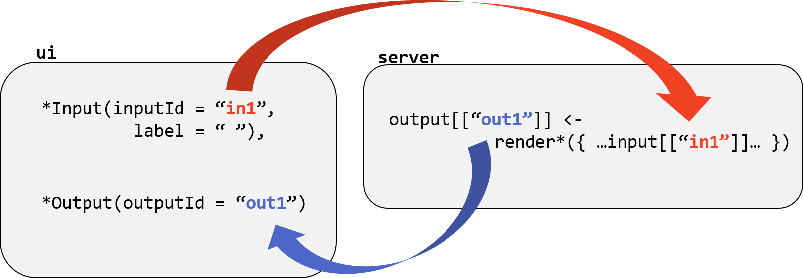
Input Objects
Input objects collect information from the user and save it into a list variable
called input. The value for any given named entity in the list updates when
the user changes the input widget with the corresponding name.
```{r, echo = FALSE}
selectInput('pick_state',
  label = 'Pick a State',
  choices = unique(cty_to_cty[['current_state']]))
```
RStudio has a nice gallery of input objects and accompanying sample code.
Contexts
As shown in the figure above, an interactive document runs R code in multiple “contexts”; for example, while rendering the document and in the connected R process running on the server. The “data” context is a special context needed for cached chunk output that we want available to the server.
```{r load_data, context = 'data', echo = FALSE, cache.extra = md5sum('worksheet.R')}
source('worksheet.R')
cty_to_cty <- subset(cty_to_cty, !is.na(movers_state_est))
```
You have to clear (i.e. delete) the cache since we added the runtime.
Output Objects
Output objects are created in the “server” context by any of several functions in the shiny package that produce output widgets.
```{r, context = 'server'}
library(dplyr)
output[['mov_plot']] <- renderPlot({
  cty_to_cty %>%
    filter(current_state == input[['pick_state']]) %>%
    group_by(prior_1year_state) %>%
    summarise(sum_new_movers = sum(movers_state_est, na.rm = TRUE)) %>%
    ggplot(aes(x = prior_1year_state, y = sum_new_movers)) +
    geom_bar(stat = 'identity') +
    theme(axis.text.x = element_text(angle = 90, hjust = 1))
})
```
```{r, echo = FALSE}
plotOutput('mov_plot')
```
Render Functions
Key functions for creating output objects:
renderPrint()renderText()renderPlot()renderTable()renderDataTable()
Reactivity
The output objects in an interactive document have to be understood in terms of
reactivity: a reactive object “knows” which changes in the environment (in
particular the list called input) should trigger it to update its value. A
useful type of user-created reactive object for an efficient pipeline is any
result of a complicated data manipulation, which can be calculated once and used
multiple times.
Create additional environment-aware objects with reactive() from the
shiny package.
```{r, context = 'server'}
plot_data <- reactive({
    filter(cty_to_cty, current_state == input[['pick_state']]) %>%
    group_by(prior_1year_state) %>%
    summarise(sum_new_movers = sum(movers_state_est, na.rm = TRUE))
})
output[['react_mov_plot']] <- renderPlot({
  plot_data() %>%
    ggplot(aes(x = prior_1year_state, y = sum_new_movers)) +
       geom_bar(stat = 'identity') +
       theme(axis.text.x = element_text(angle = 90, hjust = 1))
})
```
Don’t forget to include your plot in the document!
```{r, echo = FASE}
plotOutput('react_mov_plot')
```
In the worked example, the step of filtering the cty_to_cty data frame still only
occurs once. In a scenario where the subset of states were used for multiple
computations or vizualitions, creating the reactive plot_data() object makes
a more efficient pipeline.
Resources
Exercises
Exercise 1
Create a table with two columns, starting with a header row with fields “Character” and “Example”. Fill in the table with rows for the special Markdown characters *, **, \^, and ~, providing an example of each.
Exercise 2
Display a copy of your presentation on GitHub. Your repository on GitHub includes a free web hosting service known as GitHub Pages. Publish your worksheet there with the following steps.
- Remove any bits of the shiny runtime (GitHub only serves static pages).
- Copy the HTML output file to
docs/index.html. - Stage, commit & push the
docs/index.htmlfile to GitHub. - On GitHub, under Settings > GitHub Pages, set
docs/as the source.
Solutions
Solution 1
character | format
----------|----------
*         | *italics*
**        | **bold**
^         | super^script^
~~        | ~~strikethrough~~
Solution 2

SpaceX
If you need to catch-up before a section of code will work, just squish it's 🍅 to copy code above it into your clipboard. Then paste into your interpreter's console, run, and you'll be ready to start in on that section. Code copied by both 🍅 and 📋 will also appear below, where you can edit first, and then copy, paste, and run again.
# Nothing here yet!