Introduction to Land Change Modelling
Lesson 2 with Benoit Parmentier
Contents
####################################   Land Use and Land Cover Change   #######################################
############################  Analyze Land Cover change in Houston  #######################################
#This script performs analyses for the Exercise 4 of the Geospatial Short Course using aggregated NLCD values.
#The goal is to assess land cover change using two land cover maps in the Houston areas.
#Additional datasets are provided for the land cover change modeling. A model is built for Harris county.
#
#AUTHORS: Benoit Parmentier
#DATE CREATED: 03/16/2018
#DATE MODIFIED: 03/28/2018
#Version: 1
#PROJECT: SESYNC and AAG 2018 Geospatial Short Course
#TO DO:
#
#COMMIT: clean up code for workshop
#
#################################################################################################

###Loading R library and packages

library(sp) # spatial/geographfic objects and functions
library(rgdal) #GDAL/OGR binding for R with functionalities
rgdal: version: 1.2-18, (SVN revision 718)
 Geospatial Data Abstraction Library extensions to R successfully loaded
 Loaded GDAL runtime: GDAL 2.1.3, released 2017/20/01
 Path to GDAL shared files: /usr/share/gdal/2.1
 GDAL binary built with GEOS: TRUE
 Loaded PROJ.4 runtime: Rel. 4.9.2, 08 September 2015, [PJ_VERSION: 492]
 Path to PROJ.4 shared files: (autodetected)
 Linking to sp version: 1.2-7
library(spdep) #spatial analyses operations, functions etc.
Loading required package: Matrix
Loading required package: spData
To access larger datasets in this package, install the spDataLarge
package with: `install.packages('spDataLarge',
repos='https://nowosad.github.io/drat/', type='source'))`
library(gtools) # contains mixsort and other useful functions
library(maptools) # tools to manipulate spatial data
Checking rgeos availability: TRUE
library(parallel) # parallel computation, part of base package no
library(rasterVis) # raster visualization operations
Loading required package: raster
Loading required package: lattice
Loading required package: latticeExtra
Loading required package: RColorBrewer
library(raster) # raster functionalities
library(forecast) #ARIMA forecasting
library(xts) #extension for time series object and analyses
Loading required package: zoo
Attaching package: 'zoo'
The following objects are masked from 'package:base':

    as.Date, as.Date.numeric
library(zoo) # time series object and analysis
library(lubridate) # dates functionality
Attaching package: 'lubridate'
The following object is masked from 'package:base':

    date
library(colorRamps) #contains matlab.like color palette
library(rgeos) #contains topological operations
rgeos version: 0.3-26, (SVN revision 560)
 GEOS runtime version: 3.5.1-CAPI-1.9.1 r4246
 Linking to sp version: 1.2-5
 Polygon checking: TRUE
library(sphet) #contains spreg, spatial regression modeling
Attaching package: 'sphet'
The following object is masked from 'package:raster':

    distance
library(BMS) #contains hex2bin and bin2hex, Bayesian methods
library(bitops) # function for bitwise operations
library(foreign) # import datasets from SAS, spss, stata and other sources
#library(gdata) #read xls, dbf etc., not recently updated but useful
library(classInt) #methods to generate class limits
library(plyr) #data wrangling: various operations for splitting, combining data
Attaching package: 'plyr'
The following object is masked from 'package:lubridate':

    here
#library(gstat) #spatial interpolation and kriging methods
library(readxl) #functionalities to read in excel type data
library(psych) #pca/eigenvector decomposition functionalities
Attaching package: 'psych'
The following object is masked from 'package:gtools':

    logit
library(sf) #spatial objects and functionalities
Linking to GEOS 3.5.1, GDAL 2.1.3, proj.4 4.9.2
library(plotrix) #various graphic functions e.g. draw.circle
Attaching package: 'plotrix'
The following object is masked from 'package:psych':

    rescale
library(TOC) # TOC and ROC for raster images
Loading required package: bit
Attaching package bit
package:bit (c) 2008-2012 Jens Oehlschlaegel (GPL-2)
creators: bit bitwhich
coercion: as.logical as.integer as.bit as.bitwhich which
operator: ! & | xor != ==
querying: print length any all min max range sum summary
bit access: length<- [ [<- [[ [[<-
for more help type ?bit
Attaching package: 'bit'
The following object is masked _by_ '.GlobalEnv':

    chunk
The following object is masked from 'package:psych':

    keysort
The following object is masked from 'package:base':

    xor
library(ROCR) # ROCR general for data.frame
Loading required package: gplots
Attaching package: 'gplots'
The following object is masked from 'package:plotrix':

    plotCI
The following object is masked from 'package:stats':

    lowess
###### Functions used in this script

create_dir_fun <- function(outDir,out_suffix=NULL){
  #if out_suffix is not null then append out_suffix string
  if(!is.null(out_suffix)){
    out_name <- paste("output_",out_suffix,sep="")
    outDir <- file.path(outDir,out_name)
  }
  #create if does not exists
  if(!file.exists(outDir)){
    dir.create(outDir)
  }
  return(outDir)
}

#####  Parameters and argument set up ###########

#Separate inputs and outputs directories
in_dir_var <- "data"
out_dir <- "."

### General parameters

#NLCD coordinate reference system: we will use this projection rather than TX.
CRS_reg <- "+proj=aea +lat_1=29.5 +lat_2=45.5 +lat_0=23 +lon_0=-96 +x_0=0 +y_0=0 +ellps=GRS80 +towgs84=0,0,0,0,0,0,0 +units=m +no_defs"
file_format <- ".tif" #raster output format
NA_flag_val <- -9999 # NA value assigned to output raster
out_suffix <-"lesson2" #output suffix for the files and ouptu folder #PARAM 8
create_out_dir_param=FALSE # if TRUE, a output dir using output suffix will be created
method_proj_val <- "bilinear" # method option for the reprojection and resampling
gdal_installed <- TRUE #if TRUE, GDAL is used to generate distance files

### Input data files
rastername_county_harris <- "harris_county_mask.tif" #Region of interest: extent of Harris County
elevation_fname <- "srtm_Houston_area_90m.tif" #SRTM elevation
roads_fname <- "r_roads_Harris.tif" #Road count for Harris county

### Aggreagate NLCD input files
infile_land_cover_date1 <- "agg_3_r_nlcd2001_Houston.tif"
infile_land_cover_date2 <- "agg_3_r_nlcd2006_Houston.tif"
infile_land_cover_date3 <- "agg_3_r_nlcd2011_Houston.tif"

infile_name_nlcd_legend <- "nlcd_legend.txt"
infile_name_nlcd_classification_system <- "classification_system_nlcd_legend.xlsx"

######################### START SCRIPT ###############################

## First create an output directory to separate inputs and outputs

if(is.null(out_dir)){
  out_dir <- dirname(in_dir) #output will be created in the input dir
}

out_suffix_s <- out_suffix #can modify name of output suffix
if(create_out_dir_param==TRUE){
  out_dir <- create_dir_fun(out_dir,out_suffix_s)
  setwd(out_dir)
}else{
  setwd(out_dir) #use previoulsy defined directory
}

###########################################
### PART I: READ AND VISUALIZE DATA #######

r_lc_date1 <- raster(file.path(in_dir_var,infile_land_cover_date1)) #NLCD 2001
r_lc_date2 <- raster(file.path(in_dir_var,infile_land_cover_date2)) #NLCD 2006
r_lc_date3 <- raster(file.path(in_dir_var,infile_land_cover_date2)) #NLCD 2011

lc_legend_df <- read.table(file.path(in_dir_var,infile_name_nlcd_legend),
                           stringsAsFactors = F,
                           sep=",")

head(lc_legend_df) # Inspect data
  ID      COUNT Red Green Blue NLCD.2006.Land.Cover.Class Opacity
1  0 7854240512   0     0    0               Unclassified     255
2  1          0   0   249    0                                255
3  2          0   0     0    0                                255
4  3          0   0     0    0                                255
5  4          0   0     0    0                                255
6  5          0   0     0    0                                255
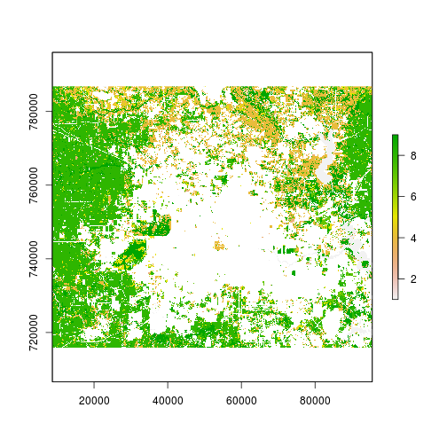
plot(r_lc_date2) # View NLCD 2006, we will need to add the legend use the appropriate palette!!
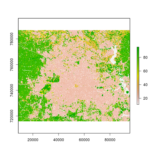
### Let's add legend and examine existing land cover categories

freq_tb_date2 <- freq(r_lc_date2)
head(freq_tb_date2) #view first 5 rows, note this is a matrix object.
     value  count
[1,]    11  18404
[2,]    21  95347
[3,]    22  93687
[4,]    23 122911
[5,]    24  53352
[6,]    31   6097
### Let's generate a palette from the NLCD legend information to view the existing land cover for 2006.
names(lc_legend_df)
[1] "ID"                         "COUNT"
[3] "Red"                        "Green"
[5] "Blue"                       "NLCD.2006.Land.Cover.Class"
[7] "Opacity"
dim(lc_legend_df) #contains a lot of empty rows
[1] 256 7
lc_legend_df<- subset(lc_legend_df,COUNT>0) #subset the data to remove unsured rows
### Generate a palette color from the input Red, Green and Blue information using RGB encoding:
lc_legend_df$rgb <- paste(lc_legend_df$Red,lc_legend_df$Green,lc_legend_df$Blue,sep=",") #combine
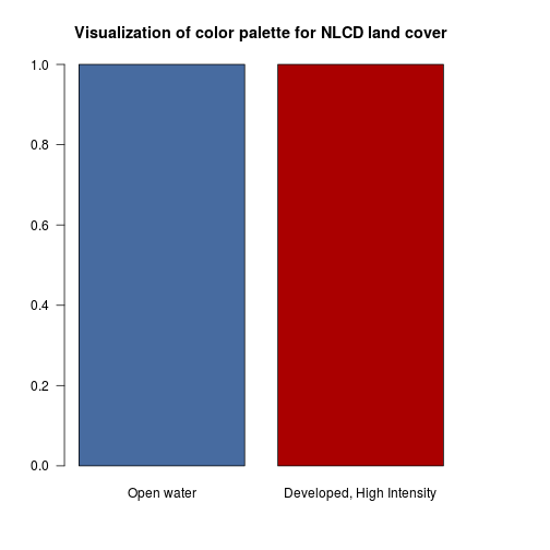
### row 2 correspond to the "open water" category
color_val_water <- rgb(lc_legend_df$Red[2],lc_legend_df$Green[2],lc_legend_df$Blue[2],maxColorValue = 255)
color_val_developed_high <- rgb(lc_legend_df$Red[7],lc_legend_df$Green[7],lc_legend_df$Blue[7],maxColorValue = 255)
lc_col_palette <- c(color_val_water,color_val_developed_high)
barplot(c(1,1),
col=lc_col_palette,
main="Visualization of color palette for NLCD land cover",
names.arg=c("Open water", "Developed, High Intensity"),las=1)
### Let's generate a color for all the land cover categories by using lapply and function
n_cat <- nrow(lc_legend_df)
lc_col_palette <- lapply(1:n_cat,
FUN=function(i){rgb(lc_legend_df$Red[i],lc_legend_df$Green[i],lc_legend_df$Blue[i],maxColorValue = 255)})
lc_col_palette <- unlist(lc_col_palette)
lc_legend_df$palette <- lc_col_palette
r_lc_date2 <- ratify(r_lc_date2) # create a raster layer with categorical information
rat <- levels(r_lc_date2)[[1]] #This is a data.frame with the categories present in the raster
lc_legend_df_date2 <- subset(lc_legend_df,lc_legend_df$ID%in% (rat[,1])) #find the land cover types present in date 2 (2006)
rat$legend <- lc_legend_df_date2$NLCD.2006.Land.Cover.Class #assign it back in case it is missing
levels(r_lc_date2) <- rat #add the information to the raster layer
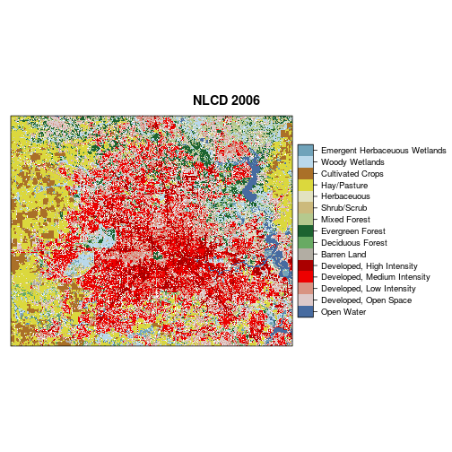
### Now generate a plot of land cover with the NLCD legend and palette
levelplot(r_lc_date2,
col.regions = lc_legend_df_date2$palette,
scales=list(draw=FALSE),
main = "NLCD 2006")
################################################
###  PART II : Analyze change and transitions

## As the plot shows for 2006, we have 15 land cover types. Analyzing such complex categories in terms of decreasse (loss), increase (gain),
# persistence in land cover will generate a large number of transitions (potential up to 15*15=225 transitions in this case!)

## To generalize the information, let's aggregate leveraging the hierachical nature of NLCD Anderson Classification system.

lc_system_nlcd_df <- read_xlsx(file.path(in_dir_var,infile_name_nlcd_classification_system))
head(lc_system_nlcd_df) #inspect data
# A tibble: 6 x 5
  id_l1 id_l2 name_l1   name_l2                     `Classification Descr~
  <dbl> <dbl> <chr>     <chr>                       <chr>
1    1.   11. Water     Open Water                  Open Water- areas of ~
2    1.   12. Water     Perennial Ice/Snow          Perennial Ice/Snow- a~
3    2.   21. Developed Developed, Open Space       Developed, Open Space~
4    2.   22. Developed Developed, Low Intensity    Developed, Low Intens~
5    2.   23. Developed Developed, Medium Intensity Developed, Medium Int~
6    2.   24. Developed Developed High Intensity    Developed High Intens~
### Let's identify existing cover and compute change:
r_stack_nlcd <- stack(r_lc_date1,r_lc_date2)
freq_tb_nlcd <- as.data.frame(freq(r_stack_nlcd,merge=T))
head(freq_tb_nlcd)
  value agg_3_r_nlcd2001_Houston agg_3_r_nlcd2006_Houston
1    11                    17800                    18404
2    21                    92135                    95347
3    22                    89035                    93687
4    23                   102053                   122911
5    24                    47830                    53352
6    31                     4540                     6097
dim(lc_system_nlcd_df) # We have categories that are not relevant to the study area and time period.
[1] 20 5
lc_system_nlcd_df <- subset(lc_system_nlcd_df,id_l2%in%freq_tb_nlcd$value )
dim(lc_system_nlcd_df) # Now 15 land categories instead of 20.
[1] 15 5
### Selectet relevant columns for the reclassification
rec_df <- lc_system_nlcd_df[,c(2,1)]
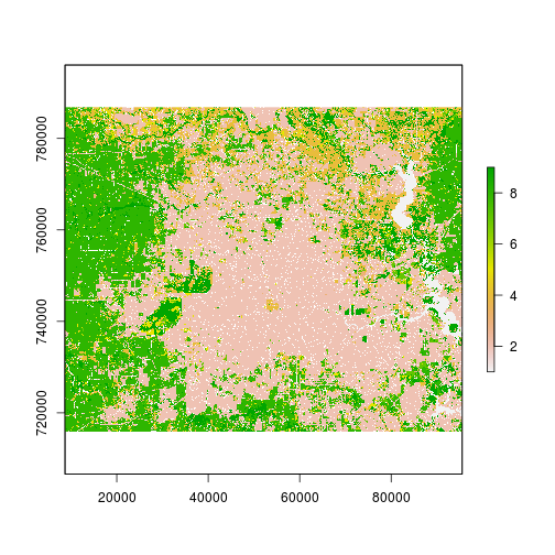
r_date1_rec <- subs(r_lc_date1,rec_df,by="id_l2","id_l1")
r_date2_rec <- subs(r_lc_date2,rec_df,by="id_l2","id_l1")
plot(r_date1_rec)
rec_xtab_df <- crosstab(r_date1_rec,r_date2_rec,long=T)
names(rec_xtab_df) <- c("2001","2011","freq")

head(rec_xtab_df)
  2001 2011  freq
1    1    1 17285
2    2    1     7
3    3    1   231
4    4    1    76
5    5    1    21
6    7    1    73
dim(rec_xtab_df) #9*9 possible transitions if we include NA values
[1] 81 3
print(rec_xtab_df) # View the full table
   2001 2011   freq
1     1    1  17285
2     2    1      7
3     3    1    231
4     4    1     76
5     5    1     21
6     7    1     73
7     8    1    306
8     9    1    302
9  <NA>    1    103
10    1    2     74
11    2    2 325161
12    3    2   1111
13    4    2  10115
14    5    2   1364
15    7    2   3243
16    8    2  12540
17    9    2   3987
18 <NA>    2   7702
19    1    3    176
20    2    3     10
21    3    3   2815
22    4    3    386
23    5    3    232
24    7    3    145
25    8    3   1929
26    9    3    314
27 <NA>    3     90
28    1    4      8
29    2    4     40
30    3    4     10
31    4    4  77877
32    5    4    192
33    7    4     27
34    8    4     48
35    9    4     41
36 <NA>    4    242
37    1    5     34
38    2    5     14
39    3    5     70
40    4    5    807
41    5    5  13782
42    7    5    752
43    8    5    264
44    9    5     87
45 <NA>    5    186
46    1    7     95
47    2    7     32
48    3    7    115
49    4    7    996
50    5    7    452
51    7    7  16967
52    8    7    411
53    9    7     91
54 <NA>    7    213
55    1    8      3
56    2    8     17
57    3    8      7
58    4    8    127
59    5    8     37
60    7    8     14
61    8    8 154887
62    9    8    110
63 <NA>    8     83
64    1    9     38
65    2    9     19
66    3    9     51
67    4    9    116
68    5    9     11
69    7    9     19
70    8    9     52
71    9    9  58478
72 <NA>    9    145
73    1 <NA>     87
74    2 <NA>   5753
75    3 <NA>    130
76    4 <NA>   1654
77    5 <NA>    271
78    7 <NA>    516
79    8 <NA>   1673
80    9 <NA>    691
81 <NA> <NA>  32745
which.max(rec_xtab_df$freq)
[1] 11
rec_xtab_df[11,] # Note the most important transition is persistence!!
   2001 2011   freq
11    2    2 325161
### Let's rank the transition:
class(rec_xtab_df)
[1] "data.frame"
is.na(rec_xtab_df$freq)
 [1] FALSE FALSE FALSE FALSE FALSE FALSE FALSE FALSE FALSE FALSE FALSE
[12] FALSE FALSE FALSE FALSE FALSE FALSE FALSE FALSE FALSE FALSE FALSE
[23] FALSE FALSE FALSE FALSE FALSE FALSE FALSE FALSE FALSE FALSE FALSE
[34] FALSE FALSE FALSE FALSE FALSE FALSE FALSE FALSE FALSE FALSE FALSE
[45] FALSE FALSE FALSE FALSE FALSE FALSE FALSE FALSE FALSE FALSE FALSE
[56] FALSE FALSE FALSE FALSE FALSE FALSE FALSE FALSE FALSE FALSE FALSE
[67] FALSE FALSE FALSE FALSE FALSE FALSE FALSE FALSE FALSE FALSE FALSE
[78] FALSE FALSE FALSE FALSE
rec_xtab_df_ranked <- rec_xtab_df[order(rec_xtab_df$freq,decreasing=T) , ]
head(rec_xtab_df_ranked) # Unsurprsingly, top transitions are persistence categories
   2001 2011   freq
11    2    2 325161
61    8    8 154887
31    4    4  77877
71    9    9  58478
81 <NA> <NA>  32745
1     1    1  17285
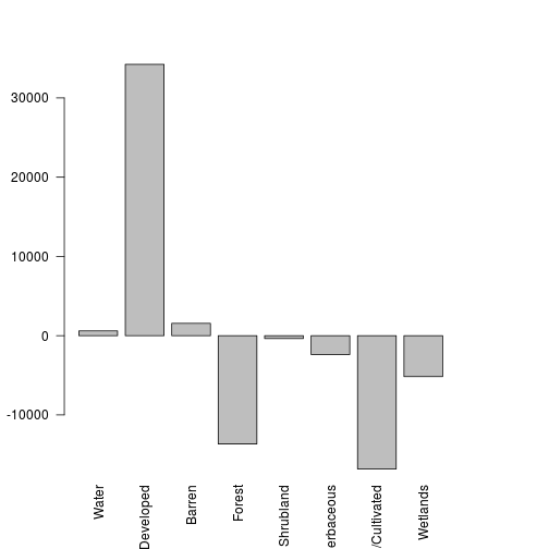
### Let's examine the overall change in categories rather than transitions

label_legend_df <- data.frame(ID=lc_system_nlcd_df$id_l1,name=lc_system_nlcd_df$name_l1)
r_stack <- stack(r_date1_rec,r_date2_rec)

lc_df <- freq(r_stack,merge=T)
names(lc_df) <- c("value","date1","date2")
lc_df$diff <- lc_df$date2 - lc_df$date1 #difference for each land cover categories over the 2001-2011 time period
head(lc_df) # Quickly examine the output
  value  date1  date2   diff
1     1  17800  18404    604
2     2 331053 365297  34244
3     3   4540   6097   1557
4     4  92154  78485 -13669
5     5  16362  15996   -366
6     7  21756  19372  -2384
### Add relevant categories
lc_df <- merge(lc_df,label_legend_df,by.x="value",by.y="ID",all.y=F)
lc_df <- lc_df[!duplicated(lc_df),] #remove duplictates
head(lc_df) # Note the overall cahnge
   value  date1  date2   diff       name
1      1  17800  18404    604      Water
2      2 331053 365297  34244  Developed
6      3   4540   6097   1557     Barren
7      4  92154  78485 -13669     Forest
10     5  16362  15996   -366  Shrubland
11     7  21756  19372  -2384 Herbaceous
#### Now visualize the overall land cover changes
barplot(lc_df$diff,names.arg=lc_df$name,las=2)
total_val  <- sum(lc_df$date1)
lc_df$perc_change <- 100*lc_df$diff/total_val
barplot(lc_df$perc_change,names.arg=lc_df$name,las=2)

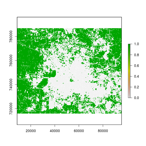
### Create a change image to map all pixels that transitioned to the developed category:

r_cat2 <- r_date2_rec==2 # developed on date 2
r_not_cat2 <- r_date1_rec!=2 #remove areas that were already developed in date1, we do not want persistence

r_change <- r_cat2 * r_not_cat2 #mask
plot(r_change,main="Land transitions to developed over 2001-2011")
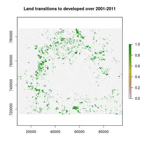
change_tb <- freq(r_change) #Find out how many pixels transitions to developed
#####################################
############# PART III: Process and Prepare variables for land change modeling ##############
## y= 1 if change to urban over 2001-2011
### Explanatory variables:
#var1: distance to existing urban in 2001
#var2: distance to road in 2001
#var3: elevation, low slope better for new development
#var4: past land cover state that may influence future land change
## 1) Generate var1 and var2 : distance to developed and distance to roads
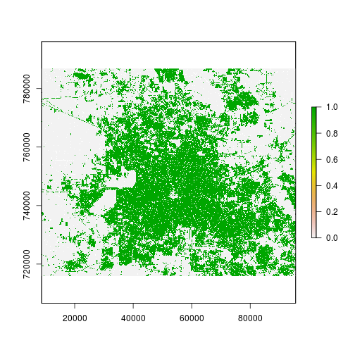
### Distance to existing in 2001: prepare information
r_cat2<- r_date1_rec==2 #developed in 2001
plot(r_cat2)
cat_bool_fname <- "developed_2001.tif" #input for the distance to road computation
writeRaster(r_cat2,filename = cat_bool_fname,overwrite=T)
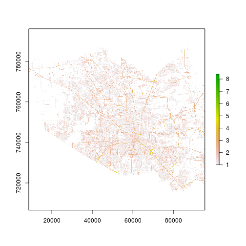
### Read in data for road count
r_roads <- raster(file.path(in_dir_var,roads_fname))
plot(r_roads,colNA="black")
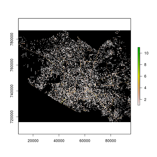
res(r_roads)
[1] 30 30
#### Aggregate to match the NLCD data resolution
r_roads_90m <- aggregate(r_roads,
                         fact=3, #factor of aggregation in x and y
                         fun=mean) #function used in aggregation values
plot(r_roads_90m)
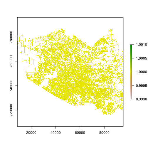
r_roads_bool <- r_roads_90m > 0
plot(r_roads_bool)
roads_bool_fname <- "roads_bool.tif" #input for the distance to road computation
writeRaster(r_roads_bool,filename = roads_bool_fname,overwrite=T)
### This part could be transformed into a function but we keep it for clarity and learning:
if(gdal_installed==TRUE){
## Distance from developed land in 2001
srcfile <- cat_bool_fname
dstfile_developed <- file.path(out_dir,paste("developed_distance_",out_suffix,file_format,sep=""))
n_values <- "1"
### Prepare GDAL command: note that gdal_proximity doesn't like when path is too long
cmd_developed_str <- paste("gdal_proximity.py",
basename(srcfile),
basename(dstfile_developed),
"-values",n_values,sep=" ")
### Distance from roads
srcfile <- roads_bool_fname
dstfile_roads <- file.path(out_dir,paste("roads_bool_distance_",out_suffix,file_format,sep=""))
n_values <- "1"
### Prepare GDAL command: note that gdal_proximity doesn't like when path is too long
cmd_roads_str <- paste("gdal_proximity.py",basename(srcfile),
basename(dstfile_roads),
"-values",n_values,sep=" ")
sys_os <- as.list(Sys.info())$sysname #Find what OS system is in use.
if(sys_os=="Windows"){
shell(cmd_developed_str)
shell(cmd_roads_str)
}else{
system(cmd_developed_str)
system(cmd_roads_str)
}
r_roads_distance <- raster(dstfile_roads)
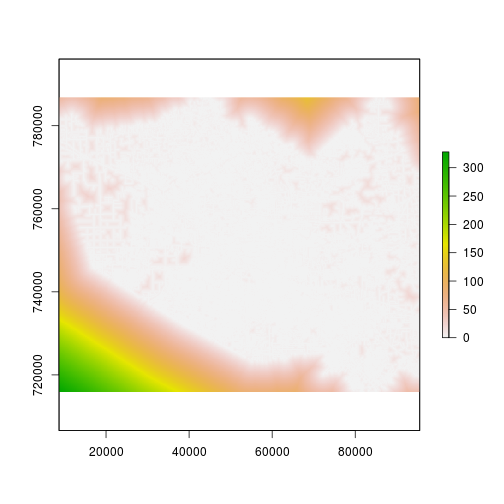
r_developed_distance <- raster(dstfile_developed)
}else{
r_developed_distance <- raster(file.path(in_dir,paste("developed_distance_",file_format,sep="")))
r_roads_distance <- raster(file.path(in_dir_var,paste("roads_bool_distance",file_format,sep="")))
}
plot(r_developed_distance) #This is at 90m.
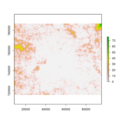
plot(r_roads_distance) #This is at 90m.
#Now rescale the distance...
min_val <- cellStats(r_roads_distance,min)
max_val <- cellStats(r_roads_distance,max)
r_roads_dist <-  (max_val - r_roads_distance) / (max_val - min_val) #high values close to 1 for areas close to roads


min_val <- cellStats(r_developed_distance,min)
max_val <- cellStats(r_developed_distance,max)
r_developed_dist <-  (max_val - r_developed_distance) / (max_val - min_val)

## 2) Generate var3 : slope
r_elevation <- raster(file.path(in_dir_var,elevation_fname))

projection(r_elevation) # This is not in the same projection as the study area.
[1] "+proj=longlat +datum=WGS84 +no_defs +ellps=WGS84 +towgs84=0,0,0"
r_elevation_reg <- projectRaster(from= r_elevation, #input raster to reproject
                                 to= r_date1_rec, #raster with desired extent, resolution and projection system
                                 method= method_proj_val) #method used in the reprojection

r_slope <- terrain(r_elevation_reg,unit="degrees")

## 3) Generate var4 : past land cover state

### reclass Land cover
r_mask <- r_date1_rec==2 #Remove developed land from
r_date1_rec_masked <- mask(r_date1_rec,r_mask,maskvalue=1)
plot(r_date1_rec_masked)
#####################################
############# PART IV: Run Model and perform assessment ##############

##############
###### Step 1: Consistent masking and generate mask removing water (1) and developed (2) in 2001

#r_mask <- (r_date1_rec!=2)*(r_date1_rec!=1)*r_county_harris
r_mask <- (r_date1_rec!=2)*(r_date1_rec!=1)
plot(r_mask)
NAvalue(r_mask) <- 0

### Read in focus area for the modeling:
r_county_harris <- raster(file.path(in_dir_var,rastername_county_harris))
### Screen for area of interest
r_mask <- r_mask * r_county_harris
r_mask[r_mask==0]<-NA
plot(r_mask)

### Check the number of NA and pixels in the study area:
tb_study_area <- freq(r_mask)
print(tb_study_area)
     value  count
[1,]     1 220338
[2,]    NA 541047
## Generate dataset for Harris county
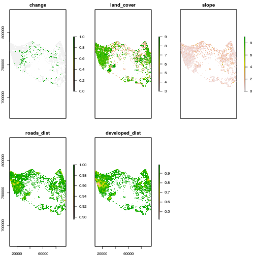
r_variables <- stack(r_change,r_date1_rec_masked,r_slope,r_roads_dist,r_developed_dist)
r_variables <- mask(r_variables,mask=r_mask) # mask to keep relevant area
names(r_variables) <- c("change","land_cover","slope","roads_dist","developed_dist")
NAvalue(r_variables) <- NA_flag_val
## Examine all the variables
plot(r_variables)
### Check for consistency in mask:
NA_freq_tb <- freq(r_variables,value=NA,merge=T)
### Notice that the number of NA is not consistent.
### Let's recombine all NA for consstencies:
plot(r_variables)
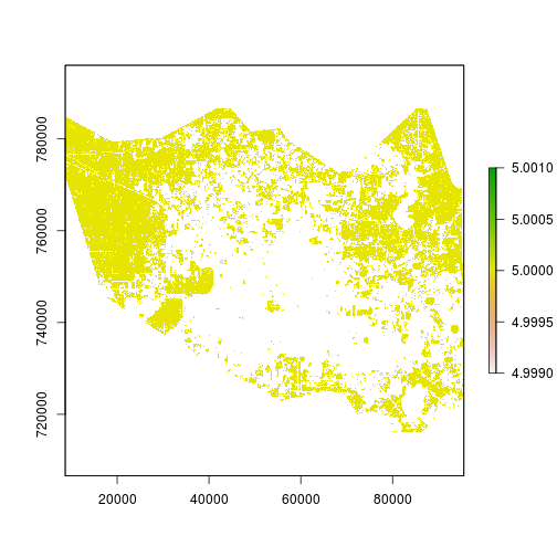
r_NA <- r_variables > -1 #There are no negative values in the raster stack
r_valid_pixels <- overlay(r_NA,fun=sum)
plot(r_valid_pixels)
dim(r_NA)
[1] 789 965 5
freq(r_valid_pixels)
     value  count
[1,]     5 215437
[2,]    NA 545948
r_mask <- r_valid_pixels > 0
r_variables <- mask(r_variables,r_mask)
#r_variables <- freq(r_test2,value=NA,merge=T)
names(r_variables) <- c("change","land_cover","slope","roads_dist","developed_dist")

###############
###### Step 2: Fit glm model and generate predictions

variables_df <- na.omit(as.data.frame(r_variables))
dim(variables_df)
[1] 215437 5
variables_df$land_cover <- as.factor(variables_df$land_cover)
variables_df$change <- as.factor(variables_df$change)

names(variables_df)
[1] "change"         "land_cover"     "slope"          "roads_dist"
[5] "developed_dist"
#names(variables_df) <- c("change","land_cover","elevation","roads_dist","developed_dist")

mod_glm <- glm(change ~ land_cover + slope + roads_dist + developed_dist,
           data=variables_df , family=binomial())
Warning: glm.fit: fitted probabilities numerically 0 or 1 occurred
print(mod_glm)
Call:  glm(formula = change ~ land_cover + slope + roads_dist + developed_dist,
    family = binomial(), data = variables_df)

Coefficients:
   (Intercept)     land_cover4     land_cover5     land_cover7
     -308.5419         -0.9241         -1.2272         -0.7449
   land_cover8     land_cover9           slope      roads_dist
       -1.0081         -1.2218         -0.2112        298.0062
developed_dist
       11.1344

Degrees of Freedom: 215436 Total (i.e. Null);  215428 Residual
Null Deviance:	    142300
Residual Deviance: 112900 	AIC: 112900
summary(mod_glm)
Call:
glm(formula = change ~ land_cover + slope + roads_dist + developed_dist,
    family = binomial(), data = variables_df)

Deviance Residuals:
    Min       1Q   Median       3Q      Max
-1.3712  -0.5328  -0.2546  -0.0418   6.6490

Coefficients:
                 Estimate Std. Error z value Pr(>|z|)
(Intercept)    -308.54187    3.05822 -100.89   <2e-16 ***
land_cover4      -0.92415    0.04763  -19.40   <2e-16 ***
land_cover5      -1.22723    0.06081  -20.18   <2e-16 ***
land_cover7      -0.74491    0.05151  -14.46   <2e-16 ***
land_cover8      -1.00809    0.04851  -20.78   <2e-16 ***
land_cover9      -1.22180    0.05087  -24.02   <2e-16 ***
slope            -0.21119    0.01307  -16.16   <2e-16 ***
roads_dist      298.00624    3.07499   96.91   <2e-16 ***
developed_dist   11.13435    0.26236   42.44   <2e-16 ***
---
Signif. codes:  0 '***' 0.001 '**' 0.01 '*' 0.05 '.' 0.1 ' ' 1

(Dispersion parameter for binomial family taken to be 1)

    Null deviance: 142342  on 215436  degrees of freedom
Residual deviance: 112871  on 215428  degrees of freedom
AIC: 112889

Number of Fisher Scoring iterations: 8
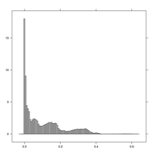
r_p <- predict(r_variables, mod_glm, type="response")
plot(r_p)
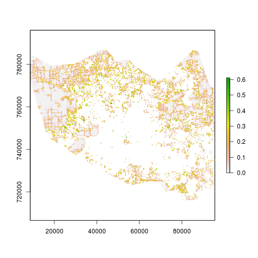
histogram(r_p)
###############
###### Step 3: Model assessment with ROC

## We use the TOC package since it allows for the use of raster layers.

r_change_harris <- subset(r_variables,"change")

## These are the inputs for the assessment
plot(r_change_harris) # boolean reference variable
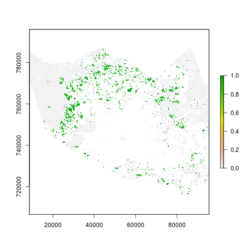
plot(r_mask) # mask for relevant observation
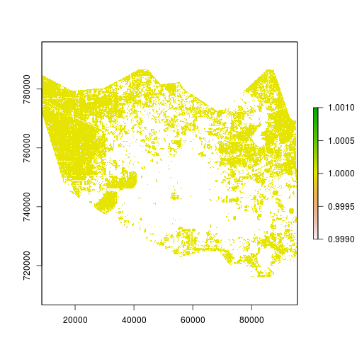
plot(r_p) # index variable to assess

roc_rast <- ROC(index=r_p,
                  boolean=r_change_harris,
                  mask=r_mask,
                  nthres=100)

plot(roc_rast)
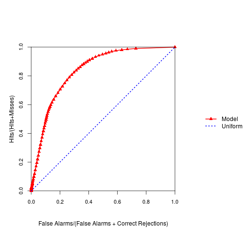
slot(roc_rast,"AUC") #this is the AUC from ROC for the logistic modeling
[1] 0.836335
toc_rast <- TOC(index=r_p,
                  boolean=r_change_harris,
                  mask=r_mask,
                  nthres=100)

plot(toc_rast)
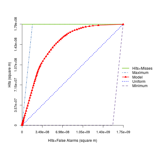
slot(toc_rast,"AUC") #this is the AUC from TOC for the logistic modeling
[1] 0.836335
############################### End of script #####################################