Leaflet in R
Lesson 8 with Kelly Hondula
Contents
- Introduction
- What’s a Leaflet?
- Layers Control
- Add data Layers
- Leaflet in shiny
- Leaflet in shiny for people in a hurry
- Summary
Introduction
Leaflet is a powerful open-source Javascript library that powers interactive maps on the web. This lesson provides an overview of using leaflet, the namesake package in R, to create “slippy” Leaflet maps from R and integrate them into RShiny apps.
Like static plotting and mapping, there lots of options for interactive mapping in R. The leaflet package is actively maintained by RStudio. Some other packages for interactive maps that build off of leaflet, or other interactive plotting libraries, are: tmap, ggiraph, rbokeh, plotly, highcharter, mapedit, mapview, leaflet.extras, and leaflet.esri.
Objectives for this lesson
- Learn how to build leaflet maps with background tiles and layered features
- Customize the appearance of point and shape layers using data attributes
- Get started using leaflet objects in RShiny
What’s a Leaflet?
leaflet produces maps have controls to zoom, pan and toggle layers on and off, and can combine local data with base layers from web mapping services.
Maps will appear in RStudio’s Viewer pane, and can also be viewed in a web browser and saved as html files.
The leaflet() function creates an empty leaflet map to which layers can be added using the pipe (%>%) operator. The addTiles() functions adds a base tiled map; by default, it uses tiles made from OpenStreetMap data. Center and set an initial zoom level the map with setView(). Switch to the “Viewer” tab in RStudio to see the result.
library(leaflet)
library(webshot)
leaflet() %>%
addTiles() %>%
setView(lng = -76.505206, lat = 38.9767231, zoom = 7)
Add a new layer with a point marker using addMarkers(), with a custom message that displays when the marker is clicked.
leaflet() %>%
addTiles() %>%
setView(lng = -76.505206, lat = 38.9767231, zoom = 7) %>%
addMarkers(lng = -76.505206, lat = 38.9767231, popup = "I am here!")
In addition to OSM, there are many other data providers that make sets of tiles available to use as basemaps. There is a R list object called providers with the names of these options.
leaflet() %>%
addProviderTiles(providers$Esri.WorldImagery) %>%
setView(lng = -76.505206, lat = 38.9767231, zoom = 7) %>%
addMarkers(lng = -76.505206, lat = 38.9767231, popup = "I am here!")
Zoom all the way out. What projection does it look like this map is using?

Read more about the intracacies of web mercator e.g. why it is considered unsuitable for geospatial intelligence purposes. Learn how to define a custom leafletCRS here or see examples.
Layers Control
Layers can be assigned to named groups which can be toggled on and off by the user. baseGroups are selected with radio buttons (can only choose one at a time), and overlayGroups get checkboxes.
To implement layers control, add group names to individual layers with the group = argument AND add the layers control layer using addLayersControl().
leaflet() %>%
addTiles(group = "OSM") %>%
addProviderTiles(providers$Esri.WorldImagery, group = "Esri World Imagery") %>%
setView(lng = -76.505206, lat = 38.9767231, zoom = 7) %>%
addMarkers(lng = -76.505206, lat = 38.9767231, popup = "I am here!", group = "SESYNC") %>%
addLayersControl(baseGroups = c("OSM", "Esri World Imagery"),
overlayGroups = c("SESYNC"),
options = layersControlOptions(collapsed = FALSE))
Another type of tile layer is avaible through many web mapping services (WMS), such as the real-time weather radar data from the Iowa Environmental Mesonet.
leaflet() %>%
addTiles() %>%
setView(lng = -76.505206, lat = 38.9767231, zoom = 5) %>%
addWMSTiles(
"http://mesonet.agron.iastate.edu/cgi-bin/wms/nexrad/n0r.cgi",
layers = "nexrad-n0r-900913",
options = WMSTileOptions(format = "image/png", transparent = TRUE),
attribution = "Weather data © 2012 IEM Nexrad"
)
or USGS topographic maps from the National Map:
nhd_wms_url <- "https://basemap.nationalmap.gov/arcgis/services/USGSTopo/MapServer/WmsServer"
leaflet() %>%
setView(lng = -111.846061, lat = 36.115847, zoom = 12) %>%
addWMSTiles(nhd_wms_url, layers = "0")
Thanks USGS! Check out more USGS Web Mapping Services, and R packages for accessing, processing, and modeling data on github.
In addition to tile layers and markers, many other map features can be added and customized with add*() functions. Refer to the help documentation (eg. ?addMiniMap) to see all of the customization options and learn the default settings.
leaflet() %>%
setView(lng = -111.846061, lat = 36.115847, zoom = 12) %>%
addWMSTiles(nhd_wms_url, layers = "0") %>%
addMiniMap(zoomLevelOffset = -4)
Add layers with common map elements and customize them with add*. Even more new features coming soon!
leaflet() %>%
setView(lng = -111.846061, lat = 36.115847, zoom = 12) %>%
addWMSTiles(nhd_wms_url, layers = "0") %>%
addMiniMap(zoomLevelOffset = -4) %>%
addGraticule() %>%
addTerminator() %>%
addMeasure() %>%
addScaleBar()
Trigger custom javascript logic with EasyButtons.
leaflet() %>%
addTiles() %>%
addEasyButton(easyButton(
icon="fa-crosshairs", title = "Locate me",
onClick=JS("function(btn, map){ map.locate({setView: true}); }")))
The fine print: Note that RStudio’s viewer pane or external window does not always behave the same as a web brower.
Add data Layers
Spatial objects (points, lines, polygons, rasters) in your R environment can also be added as map layers, provided that they have a CRS defined with a datum. Leaflet will try to make the necessary trasnformation to display your data in EPSG:3857.
Read in data using sf and raster packages. Points are from the Water Quality Portal accessed via the dataRetrieval package. County boundaries are from the Census and Watershed boundaries are from USGS.
library(sf)
library(raster)
library(dplyr)
wqp_sites <- st_read("data/wqp_sites")
Reading layer `wqp_sites' from data source `/nfs/public-data/training/wqp_sites' using driver `ESRI Shapefile'
Simple feature collection with 21268 features and 34 fields
geometry type: POINT
dimension: XY
bbox: xmin: -79.48866 ymin: 37.9026 xmax: -75.11945 ymax: 39.7225
epsg (SRID): 4326
proj4string: +proj=longlat +datum=WGS84 +no_defs
counties_md <- st_read("data/cb_2016_us_county_5m") %>%
filter(STATEFP == "24") %>% st_transform(4326)
Reading layer `cb_2016_us_county_5m' from data source `/nfs/public-data/training/cb_2016_us_county_5m' using driver `ESRI Shapefile'
Simple feature collection with 3233 features and 9 fields
geometry type: MULTIPOLYGON
dimension: XY
bbox: xmin: -179.1473 ymin: -14.55255 xmax: 179.7785 ymax: 71.35256
epsg (SRID): 4269
proj4string: +proj=longlat +datum=NAD83 +no_defs
wbd_reg2 <- st_read("data/huc250k/") %>%
filter(REG == "02") %>% st_transform(4326)
Reading layer `huc250k' from data source `/nfs/public-data/training/huc250k' using driver `ESRI Shapefile'
Simple feature collection with 2158 features and 10 fields
geometry type: POLYGON
dimension: XY
bbox: xmin: -2356125 ymin: 269700.9 xmax: 2258682 ymax: 3176995
epsg (SRID): NA
proj4string: +proj=aea +lat_1=29.5 +lat_2=45.5 +lat_0=23 +lon_0=-96 +x_0=0 +y_0=0 +datum=NAD27 +units=m +no_defs
nlcd <- raster("data/nlcd_crop.grd")
Add a polygons layer, being sure to specify the data = argument. All of the add* layers have “map” as the first argument, facilitating use of the pipe (%>%) operator, but data is not the second argument so it must be named.
leaflet() %>%
addTiles() %>%
addPolygons(data = counties_md)
Customize Polygons with border and fill colors and opacities.
leaflet() %>%
addTiles() %>%
addPolygons(data = counties_md,
color = "green",
fillColor = "gray",
fillOpacity = 0.75,
weight = 1)
Attributes can be referred to using formula syntax ~ to access attribute data from an sf object or Spatial*DataFrame. What is the difference between a popup and a label?
leaflet() %>%
addTiles() %>%
addPolygons(data = counties_md, popup = ~NAME, group = "click") %>%
addPolygons(data = counties_md, label = ~NAME, group = "hover") %>%
addLayersControl(baseGroups = c("click", "hover"))
For numeric or categorical data, create a color palette from colorbrewer using colorNumeric(), colorFactor(), colorBin(), or colorQuantile(). brewer.pal.info is a data.frame containing information about the palettes.
pal <- colorNumeric("PiYG", wbd_reg2$AREA)
leaflet() %>%
addTiles() %>%
addPolygons(data = wbd_reg2,
fillColor = ~pal(AREA),
fillOpacity = 1,
weight =1)
Add a legend (which will likely duplicate arguments from the layer that used that palette).
leaflet() %>%
addTiles() %>%
addPolygons(data = wbd_reg2,
fillColor = ~pal(AREA),
fillOpacity = 0.9,
weight =1) %>%
addLegend(pal = pal, values = wbd_reg2$AREA, title = "Watershed Area")
Add points as markers, circle markers, or customized icons.
leaflet() %>%
addTiles() %>%
addMarkers(data = wqp_sites[1:1000,], group = "markers") %>%
addCircleMarkers(data = wqp_sites[1:1000,], radius = 5, group = "circlemarkers") %>%
addLayersControl(baseGroups = c("markers", "circlemarkers"))
Display a different number of markers at each zoom level using clusterOptions on markers or circle markers layers
leaflet() %>%
addTiles() %>%
addMarkers(data = wqp_sites, clusterOptions = markerClusterOptions(),
popup = ~paste(MntrnLN, ",", OrgnztI))
Rasters can be slow to load. Be patient but also check out the maxBytes = argument if need be.
leaflet() %>%
addTiles() %>%
addRasterImage(nlcd)
Leaflet in shiny
Add even more interactivity and customization to leaflet maps by incorporating them into RShiny applications.
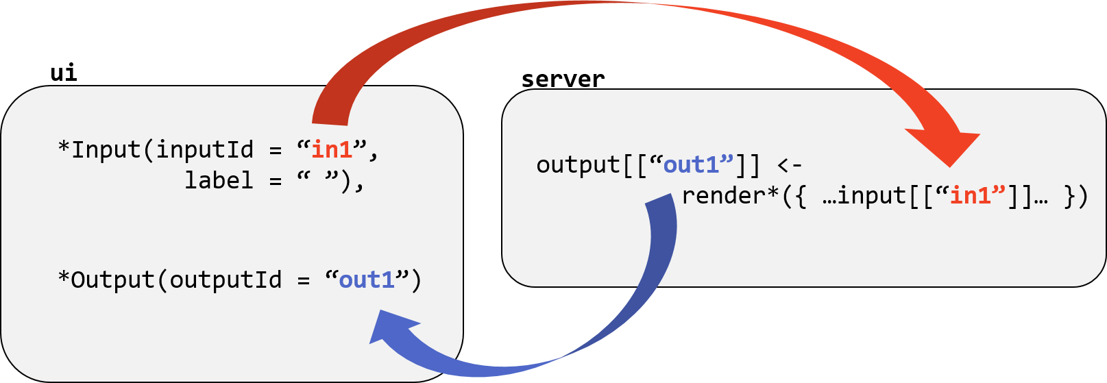
As you may have learned in the Shiny lesson, the app comprises a user interface object that defines how it appears, and a server object that defines how it behaves.
The ui and server interact through *input and *output objects such as input widgets, plots, buttons, tables, etc. Leaflet maps in Shiny are constructed with renderLeaflet() and displayed in the output using leafletOutput().

Define an output object called “map” in the server function.
output$map <- renderLeaflet({
leaflet() %>%
addTiles(group = "OSM") %>%
addProviderTiles(providers$NASAGIBS.ModisTerraTrueColorCR, group = "Modis",
options = providerTileOptions(time = "2018-01-05")) %>%
setView(lng = -76.505206, lat = 38.9767231, zoom = 7) %>%
addLayersControl(baseGroups = c("Modis", "OSM"),
options = layersControlOptions(collapsed = FALSE)
)
})
Define the ui to include the output called “map”.
ui <- fluidPage(
leafletOutput("map", height = 800)
)
Add a panel to the ui that will let users choose a calendar date.
ui <- fluidPage(
leafletOutput("map", height = 800),
absolutePanel(top = 100, right = 10, draggable = TRUE,
dateInput("dateinput", "Imagery Date", value = "2018-03-28"
)
))
Use the dateinput input object in the Provider Tiles layer.
addProviderTiles(providers$NASAGIBS.ModisTerraTrueColorCR, group = "Modis",
options = providerTileOptions(time = input$dateinput))
Leaflet in shiny for people in a hurry
Rendering maps can be slow. Use leafletProxy() so the whole map doesn’t have to be re-drawn every time the user input is updated.
Define a color palette in the server using colorNumeric and the user’s selection from the color brewer palettes (accessed via the row names of the brewer.pal.info data.frame).
pal <- colorNumeric(input$colors, wbd_reg2$AREA)
Run the app and zoom in or out. What happens when you change the color scheme?
Instead of having the input$ object referred to in the intial renderLeaflet definition in the server, move the “reactivity” to a leafletProxy() object in the server. Also redefine the initial palette in the renderLeaflet definition eg to “BrBG”.
observe({
pal <- colorNumeric(input$colors, wbd_reg2$AREA)
leafletProxy("map") %>%
clearShapes() %>% clearControls() %>%
addPolygons(data = wbd_reg2, fill = TRUE,
color = "black", weight =1,
fillColor = ~pal(AREA), fillOpacity = 0.8,
popup = ~HUC_NAME) %>%
addLegend(position = "bottomright", pal = pal, values = wbd_reg2$AREA)
})
Summary
Main functions for leaflet maps
- View window -
setView(lat, lon, zoom)fitBounds()setMaxBounds() - Background tiles -
addTiles()addProviderTiles()addWMSTiles() - Point layers -
addMarkers()addCircleMarkers()addAwesomeMarkers()addLabelOnlyMarkers() - Shape layers -
addPolylines()addCircles()addRectangles()addPolygons() - Images -
addRasterImage() - Common features -
addLegend()addLayersControl()addControl()
For Shiny apps
renderLeaflet()objects in the server and use them in the ui withleafletOutput()- Use
leafletProxy()to avoid re-rendering the whole map object