Regression
Lesson 6 with Ian Carroll
Lesson Objectives
- Learn several functions and packages for statistical modeling
- Understand the “formula” part of model specification
- Introduce increasingly complex, still “linear”, regression models
Lesson Non-objectives
Pay no attention to these very important topics.
- Experimental/sampling design
- Model validation
- Hypothesis tests
- Model comparison
Specific Achievements
- Write a
lmformula with an interaction term - Use a non-gaussian family in the
glmfunction - Add a “random effect” to a
lmerformula
Dataset
The dataset you will plot is an example of Public Use Microdata Sample (PUMS) produced by the US Census Beaurea.
library(readr)
library(dplyr)

person <- read_csv(
  file = 'data/census_pums/sample.csv',
  col_types = cols_only(
    AGEP = 'i',  # Age
    WAGP = 'd',  # Wages or salary income past 12 months
    SCHL = 'i',  # Educational attainment
    SEX = 'f',   # Sex
    OCCP = 'f',  # Occupation recode based on 2010 OCC codes
    WKHP = 'i')) # Usual hours worked per week past 12 months
This CSV file contains individuals’ anonymized responses to the 5 Year American Community Survey (ACS) completed in 2017. There are over a hundred variables giving individual level data on household members income, education, employment, ethnicity, and much more. The technical documentation provided the data definitions quoted above in comments.
Collapse the education attainment levels for this lesson, and remove non wage-earners as well as the “top coded” individuals whose income is annonymized.
person <- within(person, {
  SCHL <- factor(SCHL)
  levels(SCHL) <- list(
    'Incomplete' = c(1:15),
    'High School' = 16,
    'College Credit' = 17:20,
    'Bachelor\'s' = 21,
    'Master\'s' = 22:23,
    'Doctorate' = 24)}) %>%
  filter(
    WAGP > 0,
    WAGP < max(WAGP, na.rm = TRUE))
Formula Notation
The basic function for fitting a regression in R is the lm() function,
standing for linear model.
fit <- lm(
  formula = WAGP ~ SCHL,
  data = person)
The lm() function takes a formula argument and a data argument, and computes
the best fitting linear model (i.e. determines coefficients that minimize the
sum of squared residuals.
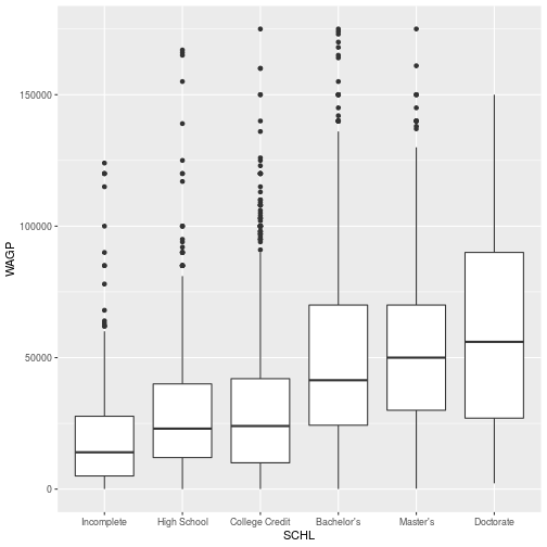
Data visualizations can help confirm intuition, but only with very simple models, typically with just one or two “fixed effects”.
> library(ggplot2)
>
> ggplot(person,
+   aes(x = SCHL, y = WAGP)) +
+   geom_boxplot()
Function, Formula, and Data
The developers of R created an approach to statistical analysis that is both concise and flexible from the users perspective, while remaining precise and well-specified for a particular fitting procedure.
The researcher contemplating a new regression analysis faces three initial challenges:
- Choose the function that implements a suitable fitting procedure.
- Write down the regression model using a formula expression combining variable names with algebra-like operators.
- Build a data frame with columns matching these variables that have suitable data types for the chosen fitting procedure.
The formula expressions are usually very concise, in part because the function chosen to implement the fitting procedure extracts much necessary information from the provided data frame. For example, whether a variable is a factor or numeric is not specified in the formula because it is specified in the data.
Formula Mini-language(s)
Across different packages in R, the formula “mini-language” has evolved to allow
complex model specification. Each package adds syntax to the formula or new
arguments to the fitting function. The lm function admits only the simplest
kinds of expressions, while the lme4 packagehas evolved this
“mini-language” to allow specification of hierarchichal models.
Linear Models
The formula requires a response variable left of a ~ and any number of
predictors to its right.
| Formula | Description |
|---|---|
y ~ a |
constant and one predictor |
y ~ a + b |
constant and two predictors |
y ~ a + b + a:b |
constant and two predictors and their interaction |
The constant (i.e. intercept) can be explicitly removed, although this is rarely needed in practice. Assume an intercept is fitted unless its absence is explicitly noted.
| Formula | Description |
|---|---|
y ~ -1 + a |
one predictor with no constant |
More or higher-order interactions are included with a shorthand that is sort of consistent with the expression’s algebraic meaning.
| Formula | Description |
|---|---|
y ~ a*b |
all combinations of two variables |
y ~ (a + b)^2 |
equivalent to y ~ a*b |
y ~ (a + b + ... )^n |
all combinations of all predictors up to order n |
Data transformation functions are allowed within the formula expression.
| Formula | Description |
|---|---|
y ~ log(a) |
log transformed variable |
y ~ sin(a) |
periodic function of a variable |
y ~ I(a*b) |
product of variables, protected by I from expansion |
The WAGP variable is always positive and includes some values that
are many orders of magnitude larger than the mean.
fit <- lm(
  log(WAGP) ~ SCHL,
  person)
> summary(fit)
Call:
lm(formula = log(WAGP) ~ SCHL, data = person)

Residuals:
    Min      1Q  Median      3Q     Max
-8.4081 -0.4712  0.2427  0.8023  2.5084

Coefficients:
                   Estimate Std. Error t value Pr(>|t|)
(Intercept)         9.21967    0.05862 157.284  < 2e-16 ***
SCHLHigh School     0.57470    0.07011   8.197 3.23e-16 ***
SCHLCollege Credit  0.58083    0.06530   8.895  < 2e-16 ***
SCHLBachelor's      1.22164    0.07245  16.862  < 2e-16 ***
SCHLMaster's        1.36922    0.08616  15.891  < 2e-16 ***
SCHLDoctorate       1.49332    0.22159   6.739 1.81e-11 ***
---
Signif. codes:  0 '***' 0.001 '**' 0.01 '*' 0.05 '.' 0.1 ' ' 1

Residual standard error: 1.19 on 4240 degrees of freedom
Multiple R-squared:  0.09518,	Adjusted R-squared:  0.09412
F-statistic: 89.21 on 5 and 4240 DF,  p-value: < 2.2e-16
Metadata Matters
For the predictors in a linear model, there is a big difference between factors and numbers.
fit <- lm(
  log(WAGP) ~ AGEP,
  person)
> summary(fit)
Call:
lm(formula = log(WAGP) ~ AGEP, data = person)

Residuals:
    Min      1Q  Median      3Q     Max
-8.8094 -0.5513  0.2479  0.8093  2.1933

Coefficients:
            Estimate Std. Error t value Pr(>|t|)
(Intercept) 8.842905   0.055483  159.38   <2e-16 ***
AGEP        0.025525   0.001226   20.81   <2e-16 ***
---
Signif. codes:  0 '***' 0.001 '**' 0.01 '*' 0.05 '.' 0.1 ' ' 1

Residual standard error: 1.191 on 4244 degrees of freedom
Multiple R-squared:  0.09261,	Adjusted R-squared:  0.0924
F-statistic: 433.2 on 1 and 4244 DF,  p-value: < 2.2e-16
The difference between 1 and 5 model degrees of freedom between the last two
summaries—with one fixed effect each—arises because SCHL is a a factor
while AGEP is numeric. In the first case you get multiple intercepts,
while in the second case you get a slope.
Generalized Linear Models
The lm function treats the response variable as numeric—the glm function
lifts this restriction and others. Not through the formula syntax, which is
the same for calls to lm and glm, but through addition of the family
argument.
GLM Families
The family argument determines the family of probability distributions in
which the response variable belongs. A key difference between families is the
data type and range.
| Family | Data Type | (default) link functions |
|---|---|---|
gaussian |
double |
identity, log, inverse |
binomial |
boolean |
logit, probit, cauchit, log, cloglog |
poisson |
integer |
log, identity, sqrt |
Gamma |
double |
inverse, identity, log |
inverse.gaussian |
double |
“1/mu^2”, inverse, identity, log |
The previous model fit with lm is (almost) identical to a model fit using
glm with the Gaussian family and identity link.
fit <- glm(log(WAGP) ~ SCHL,
    family = gaussian,
    data = person)
> summary(fit)
Call:
glm(formula = log(WAGP) ~ SCHL, family = gaussian, data = person)

Deviance Residuals:
    Min       1Q   Median       3Q      Max
-8.4081  -0.4712   0.2427   0.8023   2.5084

Coefficients:
                   Estimate Std. Error t value Pr(>|t|)
(Intercept)         9.21967    0.05862 157.284  < 2e-16 ***
SCHLHigh School     0.57470    0.07011   8.197 3.23e-16 ***
SCHLCollege Credit  0.58083    0.06530   8.895  < 2e-16 ***
SCHLBachelor's      1.22164    0.07245  16.862  < 2e-16 ***
SCHLMaster's        1.36922    0.08616  15.891  < 2e-16 ***
SCHLDoctorate       1.49332    0.22159   6.739 1.81e-11 ***
---
Signif. codes:  0 '***' 0.001 '**' 0.01 '*' 0.05 '.' 0.1 ' ' 1

(Dispersion parameter for gaussian family taken to be 1.415654)

    Null deviance: 6633.8  on 4245  degrees of freedom
Residual deviance: 6002.4  on 4240  degrees of freedom
AIC: 13533

Number of Fisher Scoring iterations: 2
- Question
- Should the coeficient estimates between this Gaussian
glm()and the previouslm()be different? - Answer
- It’s possible. The
lm()function uses a different (less general) fitting procedure than theglm()function, which uses IWLS. But with 64 bits used to store very precise numbers, it’s rare to encounter an noticeable difference in the optimum.
Logistic Regression
Calling glm with family = binomial using the default “logit” link performs
logistic regression.
fit <- glm(SEX ~ WAGP,
  family = binomial,
  data = person)
Interpretting the coefficients in the summary is non-obvious, but always works
the same way. In the person table, where men are coded as 1, the levels
function shows that 2, or women, are the first level. When using the binomial
family, the first level of the factor is consider 0 or “failure”, and all remaining
levels (typically just one) are considered 1 or “success”. The predicted value, the linear combination of variables and coeficients, is the log odds of “success”.
The positive coefficient on WAGP implies that a higher wage tilts the
prediction towards men.
> summary(fit)
Call:
glm(formula = SEX ~ WAGP, family = binomial, data = person)

Deviance Residuals:
    Min       1Q   Median       3Q      Max
-2.1479  -1.1225   0.6515   1.1673   1.3764

Coefficients:
              Estimate Std. Error z value Pr(>|z|)
(Intercept) -4.567e-01  4.906e-02  -9.308   <2e-16 ***
WAGP         1.519e-05  1.166e-06  13.028   <2e-16 ***
---
Signif. codes:  0 '***' 0.001 '**' 0.01 '*' 0.05 '.' 0.1 ' ' 1

(Dispersion parameter for binomial family taken to be 1)

    Null deviance: 5883.3  on 4245  degrees of freedom
Residual deviance: 5692.7  on 4244  degrees of freedom
AIC: 5696.7

Number of Fisher Scoring iterations: 4
The always popular indicator for goodness-of-fit is absent from the
summary of a glm result, as is the defult F-Test of the model’s significance.
The developers of glm, detecting an increase in user sophistication, are
leaving more of the model assessment up to you. The “null deviance” and
“residual deviance” provide most of the information we need. The ?anova.glm
function allows us to apply the F-test on the deviance change, although there is
a better alternative.
anova(fit, update(fit, SEX ~ 1), test = 'Chisq')
Analysis of Deviance Table

Model 1: SEX ~ WAGP
Model 2: SEX ~ 1
  Resid. Df Resid. Dev Df Deviance  Pr(>Chi)
1      4244     5692.7
2      4245     5883.3 -1  -190.51 < 2.2e-16 ***
---
Signif. codes:  0 '***' 0.001 '**' 0.01 '*' 0.05 '.' 0.1 ' ' 1
Observation Weights
Both the lm() and glm() function allow a vector of weights the same length
as the response. Weights can be necessary for logistic regression, depending on
the format of the data. The binomial family glm() works with three different
response variable formats.
factorwith only, or coerced to, two levels (binary)matrixwith two columns for the count of “successes” and “failures”numericproprtion of “successes” out ofweightstrials
Depending on your model, these three formats are not necesarilly interchangeable.
Linear Mixed Models
The lme4 package expands the formula “mini-language” to allow descriptions of “random effects”.
- normal predictors are “fixed effects”
(...|...)expressions describe “random effects”
In the context of this package, variables
added to the right of the ~ in the usual way are “fixed effects”—they
consume a well-defined number of degrees of freedom. Variables added within
(...|...) are “random effects”.
Models with random effects should be understood as specifying multiple, overlapping probability statements about the observations.
The “random intercepts” and “random slopes” models are the two most common extensions to a formula with one variable.
| Formula | Description |
|---|---|
y ~ (1 | b) + a |
random intercept for each level in b |
y ~ a + (a | b) |
random intercept and slope w.r.t. a for each level in b |
Random Intercept
The lmer function fits linear models with the lme4 extensions to
the lm formula syntax.
library(lme4)
fit <- lmer(
  log(WAGP) ~ (1|OCCP) + SCHL,
  data = person)
> summary(fit)
Linear mixed model fit by REML ['lmerMod']
Formula: log(WAGP) ~ (1 | OCCP) + SCHL
   Data: person

REML criterion at convergence: 12766.4

Scaled residuals:
    Min      1Q  Median      3Q     Max
-8.6724 -0.3421  0.2034  0.6046  2.8378

Random effects:
 Groups   Name        Variance Std.Dev.
 OCCP     (Intercept) 0.3945   0.6281
 Residual             1.0598   1.0295
Number of obs: 4246, groups:  OCCP, 380

Fixed effects:
                   Estimate Std. Error t value
(Intercept)         9.62243    0.06646 144.777
SCHLHigh School     0.34069    0.06304   5.404
SCHLCollege Credit  0.29188    0.06005   4.861
SCHLBachelor's      0.65614    0.07082   9.265
SCHLMaster's        0.88218    0.08742  10.092
SCHLDoctorate       1.04715    0.20739   5.049

Correlation of Fixed Effects:
            (Intr) SCHLHS SCHLCC SCHLB' SCHLM'
SCHLHghSchl -0.676
SCHLCllgCrd -0.736  0.752
SCHLBchlr's -0.677  0.653  0.723
SCHLMastr's -0.568  0.528  0.586  0.602
SCHLDoctort -0.232  0.218  0.242  0.242  0.247
The familiar assessment of model residuals is absent from the summary due to the lack of a widely accepted measure of null and residual deviance. The notions of model saturation, degrees of freedom, and independence of observations have all crossed onto thin ice.
In a lm or glm fit, each response is conditionally independent, given it’s
predictors and the model coefficients. Each observation corresponds to it’s own
probability statement. In a model with random effects, each response is no
longer conditionally independent, given it’s predictors and model coefficients.
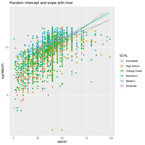
Random Slope
Adding a numeric variable on the left of a grouping specified with (...|...)
produces a “random slope” model. Here, separate coefficients for hours worked
are allowed for each level of education.
fit <- lmer(
  log(WAGP) ~ (WKHP | SCHL),
  data = person)
Warning in checkConv(attr(opt, "derivs"), opt$par, ctrl = control
$checkConv, : Model failed to converge with max|grad| = 0.207748 (tol =
0.002, component 1)
The warning that the procedure failed to converge is worth paying attention
to. In this case, we can proceed by switching to the slower numerical optimizer
that lme4 previously used by default.
fit <- lmer(
  log(WAGP) ~ (WKHP | SCHL),
  data = person,
  control = lmerControl(optimizer = "bobyqa"))
> summary(fit)
Linear mixed model fit by REML ['lmerMod']
Formula: log(WAGP) ~ (WKHP | SCHL)
   Data: person
Control: lmerControl(optimizer = "bobyqa")

REML criterion at convergence: 11670.1

Scaled residuals:
    Min      1Q  Median      3Q     Max
-9.4561 -0.3967  0.1710  0.6409  2.7948

Random effects:
 Groups   Name        Variance  Std.Dev. Corr
 SCHL     (Intercept) 11.986642 3.46217
          WKHP         0.003189 0.05647  -1.00
 Residual              0.902750 0.95013
Number of obs: 4246, groups:  SCHL, 6

Fixed effects:
            Estimate Std. Error t value
(Intercept)  11.3194     0.1052   107.6
The predict function extracts model predictions from a fitted model object
(i.e. the output of lm, glm, lmer, and gmler), providing one easy
way to visualize the effect of estimated coeficients.
ggplot(person,
  aes(x = WKHP, y = log(WAGP), color = SCHL)) +
  geom_point() +
  geom_line(aes(y = predict(fit))) +
  labs(title = 'Random intercept and slope with lmer')
Generalized Mixed Models
The glmer function adds upon lmer the option to specify the same group of
exponential family distributions for the residuals available to glm.
A Little Advice
- Don’t start with generalized linear mixed models! Work your way up through
lm()glm()lmer()glmer()
- Take time to understand the
summary()—the hazards of secondary data compel you! The vignettes for lme4 provide excellent documentation.
When stuck, ask for help on Cross Validated. If you are having trouble with lme4, who knows, Ben Bolker himself might provide the answer.
Exercises
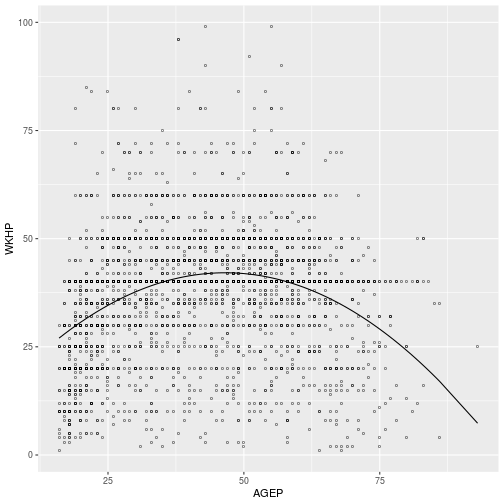
Exercise 1
Regress WKHP against AGEP, adding a second-order interaction to allow for
possible curvature in the relationship. Plot the predicted values over the data
to verify the coefficients indicate a downward quadratic relationship.
Exercise 2
Controlling for a person’s educational attainment, fit a linear model that
addresses the question of wage disparity between men and women in the U.S.
workforce. What other predictor from the person data frame would increases the
goodness-of-fit of the “control” model, before SEX is considered.
Exercise 3
Set up a generalized mixed effects model on whether a person attained an advanced degree (Master’s or Doctorate). Include sex and age as fixed effects, and include a random intercept according to occupation.
Exercise 4
Write down the formula for a random intercepts model for earned wages with a fixed effect of sex and a random effect of educational attainment.
Solutions
fit <- lm(
  WKHP ~ AGEP + I(AGEP^2),
  person)

ggplot(person,
  aes(x = AGEP, y = WKHP)) +
  geom_point(shape = 'o') +
  geom_line(aes(y = predict(fit)))
fit <- lm(WAGP ~ SCHL, person)
summary(fit)
Call:
lm(formula = WAGP ~ SCHL, data = person)

Residuals:
   Min     1Q Median     3Q    Max
-61303 -18827  -5827  12325 145173

Coefficients:
                   Estimate Std. Error t value Pr(>|t|)
(Intercept)           19614       1363  14.391  < 2e-16 ***
SCHLHigh School        8062       1630   4.945 7.89e-07 ***
SCHLCollege Credit    10214       1518   6.727 1.96e-11 ***
SCHLBachelor's        29976       1684  17.795  < 2e-16 ***
SCHLMaster's          35197       2003  17.569  < 2e-16 ***
SCHLDoctorate         43889       5152   8.519  < 2e-16 ***
---
Signif. codes:  0 '***' 0.001 '**' 0.01 '*' 0.05 '.' 0.1 ' ' 1

Residual standard error: 27660 on 4240 degrees of freedom
Multiple R-squared:  0.1389,	Adjusted R-squared:  0.1379
F-statistic: 136.8 on 5 and 4240 DF,  p-value: < 2.2e-16
The “baseline” model includes educational attainment, when compared to a model with sex as a second predictor, there is a strong indication of signifigance.
anova(fit, update(fit, WAGP ~ SCHL + SEX))
Analysis of Variance Table

Model 1: WAGP ~ SCHL
Model 2: WAGP ~ SCHL + SEX
  Res.Df        RSS Df  Sum of Sq      F    Pr(>F)
1   4240 3.2450e+12
2   4239 3.0469e+12  1 1.9806e+11 275.55 < 2.2e-16 ***
---
Signif. codes:  0 '***' 0.001 '**' 0.01 '*' 0.05 '.' 0.1 ' ' 1
Adding WKHP to the baseline increases the to .32 from .14 with just
SCHL. There is no way to include the possibility that hours worked also
dependends on sex, giving a direct and indirect path to the gender wage gap, in
a linear model.
summary(update(fit, WAGP ~ SCHL + WKHP))
Call:
lm(formula = WAGP ~ SCHL + WKHP, data = person)

Residuals:
   Min     1Q Median     3Q    Max
-82762 -14392  -3919   9306 142326

Coefficients:
                    Estimate Std. Error t value Pr(>|t|)
(Intercept)        -16510.68    1627.64 -10.144  < 2e-16 ***
SCHLHigh School      3230.58    1458.67   2.215   0.0268 *
SCHLCollege Credit   7146.98    1354.98   5.275 1.40e-07 ***
SCHLBachelor's      23865.31    1511.03  15.794  < 2e-16 ***
SCHLMaster's        27993.27    1796.83  15.579  < 2e-16 ***
SCHLDoctorate       34789.96    4595.62   7.570 4.54e-14 ***
WKHP                 1050.93      31.56  33.304  < 2e-16 ***
---
Signif. codes:  0 '***' 0.001 '**' 0.01 '*' 0.05 '.' 0.1 ' ' 1

Residual standard error: 24630 on 4239 degrees of freedom
Multiple R-squared:  0.3175,	Adjusted R-squared:  0.3165
F-statistic: 328.6 on 6 and 4239 DF,  p-value: < 2.2e-16
df <- person
levels(df$SCHL) <- c(0, 0, 0, 0, 1, 1)
fit <- glmer(
  SCHL ~ (1 | OCCP) + AGEP,
  family = binomial,
  data = df)
anova(fit, update(fit, . ~ . + SEX), test = 'Chisq')
Data: df
Models:
fit: SCHL ~ (1 | OCCP) + AGEP
update(fit, . ~ . + SEX): SCHL ~ (1 | OCCP) + AGEP + SEX
                         Df    AIC    BIC  logLik deviance  Chisq Chi Df
fit                       3 1996.5 2015.6 -995.27   1990.5
update(fit, . ~ . + SEX)  4 1997.6 2023.0 -994.79   1989.6 0.9572      1
                         Pr(>Chisq)
fit
update(fit, . ~ . + SEX)     0.3279
WAGP ~ (1 | SCHL) + SEX
WAGP ~ (1 | SCHL) + SEX
If you need to catch-up before a section of code will work, just squish it's 🍅 to copy code above it into your clipboard. Then paste into your interpreter's console, run, and you'll be ready to start in on that section. Code copied by both 🍅 and 📋 will also appear below, where you can edit first, and then copy, paste, and run again.
# Nothing here yet!