Online Data with R
Lesson 6 with Quentin Read
Lesson Objectives
- Distinguish three ways of acquiring online data
- Break down how web services use HTTP
- Learn R tools for data acquisition
Specific Achievements
- Programatically acquire data embedded in a web page
- Request data through a REST API
- Use the tidycensus package to acquire data
- Use SQLite for caching
Why script data acquisition?
- Too time intensive to acquire manually
- Integrate updated or new data
- Reproducibility
- There’s an API between you and the data
Acquiring Online Data
Data is available on the web in many different forms. How difficult is it to acquire that data to run analyses? It depends which of three approaches the data source requires:
- Web scraping
- Web service (API)
- Specialized package (API wrapper)
Web Scraping 🙁
A web browser reads HTML and JavaScript and displays a human readable page. In contrast, a web scraper is a program (a “bot”) that reads HTML and JavaScript and stores the data.
Web Service (API) 😉
API stands for Application Programming Interface (API, as opposed to GUI) that is compatible with passing data around the internet using HTTP (Hyper-text Transfer Protocol). This is not the fastest protocol for moving large datasets, but it is universal (it underpins web browsers, after all).
Specialized Package 😂
Major data providers can justify writing a “wrapper” package for their API, specific to yourlanguage of choice (e.g. Python or R), that facilitates accessing the data they provide through a web service. Sadly, not all do so.
Web Scraping
That “http” at the beginning of the URL for a possible data source is a protocol—an understanding between a client and a server about how to communicate. The client could either be a web browser or your web scraping program written in R, as long as it uses the correct protocol. After all, servers exist to serve.
The following example uses the httr and rvest packages to issue a HTTP request and handle the response.
The page we are scraping, http://research.jisao.washington.edu/pdo/PDO.latest, deals with the Pacific Decadal Oscillation (PDO), a periodic switching between warm and cool water temperatures in the northern Pacific Ocean. Specifically, it contains monthly values from 1900-2018 indicating how far above or below normal the sea surface temperature across the northern Pacific Ocean was during that month.
library(httr)

response <- GET('http://research.jisao.washington.edu/pdo/PDO.latest')
response
Response [http://research.jisao.washington.edu/pdo/PDO.latest]
  Date: 2020-07-15 12:22
  Status: 200
  Content-Type: <unknown>
  Size: 12.3 kB
<BINARY BODY>
The response is binary (0s and 1s). The rvest package translates
the raw content into an HTML document, just like a browser does. We use the
read_html function to do this.
library(rvest)

pdo_doc <- read_html(response)
pdo_doc
{html_document}
<html>
[1] <body><p>PDO INDEX\n\nIf the columns of the table appear without formatti ...
If you look at the HTML document, you can see that all the data is inside an
element called "p". We use the html_node function to extract the
single "p" element from the HTML document, then the html_text function
to extract the text from that element.
pdo_node <- html_node(pdo_doc, "p")
pdo_text <- html_text(pdo_node)
Now we have a long text string containing all the data. We can use text mining tools
like regular expressions to pull out data. If we want the twelve monthly
values for the year 2017, we can use the stringr package to get
all the text between the strings “2017” and “2018” with str_match.
library(stringr)
pdo_text_2017 <- str_match(pdo_text, "(?<=2017).*.(?=\\n2018)")
Then extract all the numeric values in the substring with str_extract_all.
str_extract_all(pdo_text_2017[1], "[0-9-.]+")
[[1]]
 [1] "0.77" "0.70" "0.74" "1.12" "0.88" "0.79" "0.10" "0.09" "0.32" "0.05"
[11] "0.15" "0.50"
You can learn more about how to use regular expressions to extract information from text strings in SESYNC’s text mining lesson.
Manual web scraping is hard!
Pages designed for humans are increasingly harder to parse programmatically.
- Servers provide different responses based on client “metadata”
- JavaScript often needs to be executed by the client
- The HTML
<table>is drifting into obscurity (mostly for the better)
HTML Tables
Sites with easily accessible html tables nowadays may be specifically intended to be parsed programmatically, rather than browsed by a human reader. The US Census provides some documentation for their data services in a massive table:
https://api.census.gov/data/2017/acs/acs5/variables.html
html_table() converts the html table into an R
data frame. Set fill = TRUE so that inconsistent numbers
of columns in each row are filled in.
census_vars_doc <- read_html('https://api.census.gov/data/2017/acs/acs5/variables.html')

table_raw <- html_node(census_vars_doc, 'table')

# This line takes a few moments to run.
census_vars <- html_table(table_raw, fill = TRUE)
> head(census_vars)
             Name           Label                                   Concept
1 25110 variables 25110 variables                           25110 variables
2          AIANHH       Geography
3          AIHHTL       Geography
4           AIRES       Geography
5            ANRC       Geography
6     B00001_001E Estimate!!Total UNWEIGHTED SAMPLE COUNT OF THE POPULATION
         Required      Attributes           Limit    Predicate Type
1 25110 variables 25110 variables 25110 variables   25110 variables
2    not required                               0 (not a predicate)
3    not required                               0 (not a predicate)
4    not required                               0 (not a predicate)
5    not required                               0 (not a predicate)
6    not required    B00001_001EA               0               int
            Group              NA
1 25110 variables 25110 variables
2             N/A            <NA>
3             N/A            <NA>
4             N/A            <NA>
5             N/A            <NA>
6          B00001            <NA>
We can use our tidy data tools to search this unwieldy documentation for variables of interest.
The call to set_tidy_names() is necessary because the table
extraction results in some columns with undefined names—a
common occurrence when parsing Web content.
library(tidyverse)

census_vars %>%
  set_tidy_names() %>%
  select(Name, Label) %>%
  filter(grepl('Median household income', Label))
           Name
1   B19013_001E
2  B19013A_001E
3  B19013B_001E
4  B19013C_001E
5  B19013D_001E
6  B19013E_001E
7  B19013F_001E
8  B19013G_001E
9  B19013H_001E
10 B19013I_001E
11  B19049_001E
12  B19049_002E
13  B19049_003E
14  B19049_004E
15  B19049_005E
16  B25099_001E
17  B25099_002E
18  B25099_003E
19  B25119_001E
20  B25119_002E
21  B25119_003E
                                                                                                                         Label
1                                 Estimate!!Median household income in the past 12 months (in 2017 inflation-adjusted dollars)
2                                 Estimate!!Median household income in the past 12 months (in 2017 inflation-adjusted dollars)
3                                 Estimate!!Median household income in the past 12 months (in 2017 inflation-adjusted dollars)
4                                 Estimate!!Median household income in the past 12 months (in 2017 inflation-adjusted dollars)
5                                 Estimate!!Median household income in the past 12 months (in 2017 inflation-adjusted dollars)
6                                 Estimate!!Median household income in the past 12 months (in 2017 inflation-adjusted dollars)
7                                 Estimate!!Median household income in the past 12 months (in 2017 inflation-adjusted dollars)
8                                 Estimate!!Median household income in the past 12 months (in 2017 inflation-adjusted dollars)
9                                 Estimate!!Median household income in the past 12 months (in 2017 inflation-adjusted dollars)
10                                Estimate!!Median household income in the past 12 months (in 2017 inflation-adjusted dollars)
11                         Estimate!!Median household income in the past 12 months (in 2017 inflation-adjusted dollars)!!Total
12    Estimate!!Median household income in the past 12 months (in 2017 inflation-adjusted dollars)!!Householder under 25 years
13    Estimate!!Median household income in the past 12 months (in 2017 inflation-adjusted dollars)!!Householder 25 to 44 years
14    Estimate!!Median household income in the past 12 months (in 2017 inflation-adjusted dollars)!!Householder 45 to 64 years
15 Estimate!!Median household income in the past 12 months (in 2017 inflation-adjusted dollars)!!Householder 65 years and over
16                                                                                    Estimate!!Median household income!!Total
17                                 Estimate!!Median household income!!Total!!Median household income for units with a mortgage
18                              Estimate!!Median household income!!Total!!Median household income for units without a mortgage
19                         Estimate!!Median household income in the past 12 months (in 2017 inflation-adjusted dollars)!!Total
20      Estimate!!Median household income in the past 12 months (in 2017 inflation-adjusted dollars)!!Owner occupied (dollars)
21     Estimate!!Median household income in the past 12 months (in 2017 inflation-adjusted dollars)!!Renter occupied (dollars)
Web Services
The US Census Bureau provides access to its vast stores of demographic data over the Web via their API at https://api.census.gov.
The I in GUI is for interface—it’s the same in API, where buttons and drop-down menus are replaced by functions and object attributes.
Instead of interfacing with a user, this kind of interface is suitable for use in programming another software application. In the case of the Census, the main component of the application is some relational database management system. There are several GUIs designed for humans to query the Census database; the Census API is meant for communication between your program (i.e. script) and their application.
You’ll often see the acronym “REST API.” In this context, REST stands for Representational state transfer. This refers to a set of standards that help ensure that the Web service works well with any computer system it may interact with.
The following code acquires data from the US Census Bureau’s American Community Survey (ACS). The ACS is a yearly survey that provides detailed population and housing information at fine geographic scale across the United States. ACS5 refers to a five-year average of the annual surveys.
Look carefully at this URL.
The URL is a query to the US Census API. The parameters after the ?
request the variable NAME for all counties in state 24 (Maryland).
In a web service, the already universal system for transferring data over the internet, known as HTTP, is half of the interface. All you really need is documentation for how to construct the URL in a standards-compliant way that the service will recognize.
| Section | Description |
|---|---|
https:// |
scheme |
api.census.gov |
authority, or simply domain if there’s no user authentication |
/data/2018/acs/acs5 |
path to a resource within a hierarchy |
? |
beginning of the query component of a URL |
get=NAME |
first query parameter |
& |
query parameter separator |
for=county:* |
second query parameter |
& |
query parameter separator |
in=state:24 |
third query parameter |
# |
beginning of the fragment component of a URL |
irrelephant |
a document section, it isn’t even sent to the server |
To construct the URL in R and send the query to the API, use GET() from
httr.
The first argument to GET() is the base URL, and the
query argument is a named list that can use to pass
the parameters of the query to the API. All the elements
of the list should be character strings.
path <- 'https://api.census.gov/data/2018/acs/acs5'
query_params <- list('get' = 'NAME,B19013_001E',
                     'for' = 'county:*',
                     'in' = 'state:24')

response = GET(path, query = query_params)
response
Response [https://api.census.gov/data/2018/acs/acs5?get=NAME%2CB19013_001E&for=county%3A%2A&in=state%3A24]
  Date: 2020-07-15 12:31
  Status: 200
  Content-Type: application/json;charset=utf-8
  Size: 1.25 kB
[["NAME","B19013_001E","state","county"],
["Worcester County, Maryland","61145","24","047"],
["Baltimore city, Maryland","48840","24","510"],
["Talbot County, Maryland","67204","24","041"],
["Harford County, Maryland","85942","24","025"],
["Howard County, Maryland","117730","24","027"],
["Anne Arundel County, Maryland","97810","24","003"],
["Baltimore County, Maryland","74127","24","005"],
["Calvert County, Maryland","104301","24","009"],
["Garrett County, Maryland","49619","24","023"],
...
Response Header
The response from the API is a bunch of 0s and 1s, but part of the HTTP protocol is to include a “header” with information about how to decode the body of the response.
Most REST APIs return as the “content” either:
- Javascript Object Notation (JSON)
- a UTF-8 encoded string of key-value pairs, where values may be lists
- e.g.
{'a':24, 'b': ['x', 'y', 'z']}
- eXtensible Markup Language (XML)
- a nested
<tag></tag>hierarchy serving the same purpose
- a nested
The header from Census says the content type is JSON.
response$headers['content-type']
$`content-type`
[1] "application/json;charset=utf-8"
Response Content
First, use httr::content() to retrieve
the JSON content of the response. Use as = 'text' to
get the content as a character vector. Then use
jsonlite::fromJSON() to convert to tabular format.
library(jsonlite)
county_income <- response %>%
  content(as = 'text') %>%
  fromJSON()
> head(county_income)
     [,1]                         [,2]          [,3]    [,4]
[1,] "NAME"                       "B19013_001E" "state" "county"
[2,] "Worcester County, Maryland" "61145"       "24"    "047"
[3,] "Baltimore city, Maryland"   "48840"       "24"    "510"
[4,] "Talbot County, Maryland"    "67204"       "24"    "041"
[5,] "Harford County, Maryland"   "85942"       "24"    "025"
[6,] "Howard County, Maryland"    "117730"      "24"    "027"
Notice that the matrix created by fromJSON() does not recognize that the first
row is a header, resulting in all columns being classified as
character. This is a typical situation when parsing Web content, and would require
API Keys & Limits
Most servers request good behavior, others enforce it.
- Size of single query
- Rate of queries (calls per second, or per day)
- User credentials specified by an API key
From the Census FAQ What Are the Query Limits?:
You can include up to 50 variables in a single API query and can make up to 500 queries per IP address per day… Please keep in mind that all queries from a business or organization having multiple employees might employ a proxy service or firewall. This will make all of the users of that business or organization appear to have the same IP address.
Specialized Packages
The third tier of access to online data is much preferred, if it exists: a dedicated package in your programming language’s repository, CRAN or PyPI.
- Additional guidance on query parameters
- Returns data in native formats
- Handles all “encoding” problems
The tidycensus package, developed by Kyle Walker, streamlines access to the API and is integrated with tidyverse packages.
To repeat the exercise below at home, request an API key at
https://api.census.gov/data/key_signup.html, and store it in a file named census_api_key.R
in your working directory. The file should contain the line
Sys.setenv(CENSUS_API_KEY = 'your many digit key'). This creates a hidden
system variable containing the key. This is good practice—it is much safer than
pasting the API key directly into your code or saving it as a variable in the global environment.
library(tidycensus)
> source('census_api_key.R')
Compared to using the API directly via the httr package:
Pros
- More concise code, quicker development
- Package documentation (if present) is usually more user-friendly than API documentaion.
- May allow seamless update if API changes
Cons
- No guarantee of updates
- Possibly limited in scope
Query the Census ACS5 survey for the variable B19013_001E (median annual household income,
in dollars) and each entity’s NAME.
variables <- c('NAME', 'B19013_001E')
Get the variables NAME and B19013_001E (median household income)
from all counties in Maryland. tidycensus
converts the JSON string into a data frame. (No need to check headers.)
This code uses the get_acs function, which is the main function in
tidycensus for interacting with the American Community Survey
API. The arguments are fairly self-explanatory. We can use the text
abbreviation for the state of Maryland (MD); the function automatically
converts this into the numerical FIPS code. The geometry = TRUE argument
means that we want get_acs output to include the county boundaries as a
spatial object.
county_income <- get_acs(geography = 'county',
                         variables = variables,
                         state = 'MD',
                         year = 2018,
                         geometry = TRUE)
> head(county_income)
Simple feature collection with 6 features and 5 fields
geometry type:  MULTIPOLYGON
dimension:      XY
bbox:           xmin: -79.06756 ymin: 38.31653 xmax: -75.70736 ymax: 39.72304
CRS:            4269
Warning: `...` is not empty.

We detected these problematic arguments:
* `needs_dots`

These dots only exist to allow future extensions and should be empty.
Did you misspecify an argument?
# A tibble: 6 x 6
  GEOID NAME        variable estimate   moe                             geometry
  <chr> <chr>       <chr>       <dbl> <dbl>                   <MULTIPOLYGON [°]>
1 24001 Allegany C… B19013_…    44065  1148 (((-79.06756 39.47944, -79.06003 39…
2 24003 Anne Arund… B19013_…    97810  1299 (((-76.84036 39.10314, -76.83678 39…
3 24005 Baltimore … B19013_…    74127   922 (((-76.3257 39.31397, -76.32452 39.…
4 24009 Calvert Co… B19013_…   104301  3548 (((-76.70121 38.71276, -76.69915 38…
5 24011 Caroline C… B19013_…    54956  2419 (((-76.01505 38.72869, -76.01321 38…
6 24013 Carroll Co… B19013_…    93363  1867 (((-77.31151 39.63914, -77.30972 39…
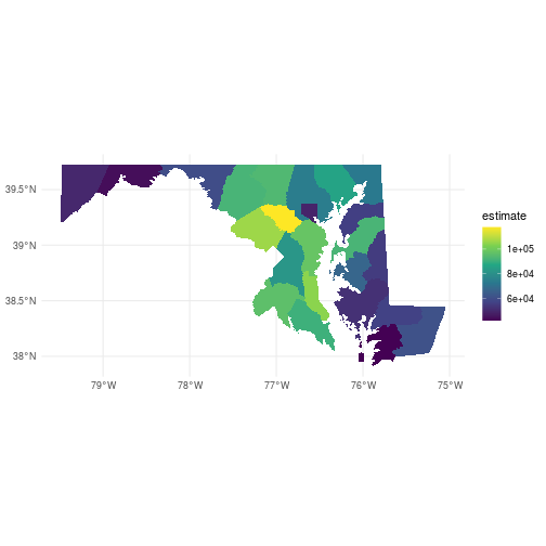
We can use dplyr to manipulate the output, and ggplot2 to visualize the data.
Because we set geometry = TRUE, tidycensus even includes spatial information in its
output that we can use to create maps!
This code uses the spatial data frame output from get_acs to plot the counties of Maryland with
fill color corresponding to the median household income of the counties, with some additional
graphical options.
ggplot(county_income) +
  geom_sf(aes(fill = estimate), color = NA) +
  coord_sf() +
  theme_minimal() +
  scale_fill_viridis_c()
For a more in-depth tutorial on R’s geospatial data types, check out SESYNC’s lesson on geospatial packages in R.
Paging & Stashing
A common strategy that web service providers take to balance their load is to limit the number of records a single API request can return. The user ends up having to flip through “pages” with the API, handling the response content at each iteration. Options for stashing data are:
- Store it all in memory, write to file at the end.
- Append each response to a file, writing frequently.
- Offload these decisions to database management software.
The data.gov API provides a case in point. Data.gov is a service provided by the U.S. federal government to make data available from across many government agencies. It hosts a catalog of raw data and of many other APIs from across government. Among the APIs catalogued by data.gov is the FoodData Central API. The U.S. Department of Agriculture maintains a data system of nutrition information for thousands of foods. We might be interested in the relative nutrient content of different fruits.
To repeat the exercise below at home, request an API key at
https://api.data.gov/signup/, and store it in a file named datagov_api_key.R
in your working directory. The file should contain the line
Sys.setenv(DATAGOV_KEY = 'your many digit key').
Load the DATAGOV_KEY variable as a system variable by importing it from the file you saved it in.
> source('datagov_api_key.R')
Run an API query for all foods with "fruit" in their name and parse the content of the response.
Just like we did previously in this lesson, we create a named list
of query parameters, including the API key and the
search string, and pass them to GET(). We use the pipe operator %>%
to pipe the output of GET() to content(). We use the as = 'parsed'
argument to convert the JSON content to a nested list.
api <- 'https://api.nal.usda.gov/fdc/v1/'
path <- 'foods/search'

query_params <- list('api_key' = Sys.getenv('DATAGOV_KEY'),
                     'query' = 'fruit')

doc <- GET(paste0(api, path), query = query_params) %>%
  content(as = 'parsed')
Extract data from the returned JSON object, which gets mapped to an
R list called doc.
First inspect the names of the list elements.
> names(doc)
[1] "foodSearchCriteria" "totalHits"          "currentPage"
[4] "totalPages"         "foods"
We can print the value of doc$totalHits to see
how many foods matched our search term, "fruit".
> doc$totalHits
[1] 18801
The claimed number of results is much larger than the length
of the foods array contained in this response. The query returned only the
first page, with 50 items.
> length(doc$foods)
[1] 50
Continue to inspect the returned object. Extract one element from the list
of foods and view its description.
> fruit <- doc$foods[[1]]
> fruit$description
[1] "Fruit leather and fruit snacks candy"
The map_dfr function from the purrr package extracts the name and
value of all the nutrients in the foodNutrients list within the first search
result, and creates a data frame.
nutrients <- map_dfr(fruit$foodNutrients,
                     ~ data.frame(name = .$nutrientName,
                                  value = .$value))
> head(nutrients, 10)
                           name  value
1                       Protein   0.55
2             Total lipid (fat)   2.84
3   Carbohydrate, by difference  84.31
4                        Energy 365.00
5                Alcohol, ethyl   0.00
6                         Water  11.25
7                      Caffeine   0.00
8                   Theobromine   0.00
9  Sugars, total including NLEA  53.37
10         Fiber, total dietary   0.00
The DBI and RSQLite packages together allow R to connect to a
database-in-a-file. If the fruits.sqlite file does not exist
in your working directory already when you try to connect,
dbConnect() will create it.
library(DBI)
library(RSQLite)

fruit_db <- dbConnect(SQLite(), 'fruits.sqlite')
Add a new pageSize parameter by appending a named element
to the existing query_params list, to request 100 documents per page.
query_params$pageSize <- 100
We will send 10 queries to the API to get 1000 total records.
In each request (each iteration through the loop),
advance the query parameter pageNumber by one.
The query will retrieve 100 records, starting with pageNumber * pageSize.
We use some tidyr and dplyr manipulations to
extract the ID number, name, and the amount of sugar from each
of the foods in the page of results returned by the query. The series of
unnest_longer() and unnest_wider() functions turns the nested list into
a data frame by successively converting lists into columns in the data frame.
This long manipulation is necessary because R does not easily handle the
nested list structures that APIs return. If we were using
a specialized API R package, typically it would handle this data wrangling
for us. After converting the list to a data frame, we use filter to retain
only the rows where the nutrientName contains the substring 'Sugars, total'
and then select the three columns we want to keep: the numerical ID of
the food, its full name, and its sugar content. Finally the 100-row data
frame is assigned to the object values.
Each time through the loop, insert the next 100 fruits
(the three-column data frame values)
in bulk to the database with dbWriteTable().
for (i in 1:10) {
  # Advance page and query
  query_params$pageNumber <- i
  response <- GET(paste0(api, path), query = query_params)
  page <- content(response, as = 'parsed')

  # Convert nested list to data frame
  values <- tibble(food = page$foods) %>%
    unnest_wider(food) %>%
    unnest_longer(foodNutrients) %>%
    unnest_wider(foodNutrients) %>%
    filter(grepl('Sugars, total', nutrientName)) %>%
    select(fdcId, description, value) %>%
    setNames(c('foodID', 'name', 'sugar'))

  # Stash in database
  dbWriteTable(fruit_db, name = 'Food', value = values, append = TRUE)

}
View the records in the database by reading
everything we have so far into a data frame
with dbReadTable().
fruit_sugar_content <- dbReadTable(fruit_db, name = 'Food')
> head(fruit_sugar_content, 10)
   foodID                                       name sugar
1  789246       Fruit leather and fruit snacks candy 53.37
2  781278 Fruit smoothie, with whole fruit and dairy  8.28
3  786863 Fruit smoothie, with whole fruit, no dairy  8.20
4  789150                                Fruit sauce 36.23
5  786838                                Soup, fruit 14.77
6  789114                                Fruit syrup 53.00
7  784748                               Bread, fruit 24.96
8  167781                              Candied fruit 80.68
9  784768                      Cheesecake with fruit 15.27
10 784566                           Croissant, fruit 13.98
Don’t forget to disconnect from your database!
dbDisconnect(fruit_db)
Takeaway
-
Web scraping is hard and unreliable, but sometimes there is no other option.
-
Web services are the most common resource.
-
Use a package specific to your API if one is available.
Web services do not always have great documentation—what parameters are acceptable or necessary may not be clear. Some may even be poorly documented on purpose if the API wasn’t designed for public use! Even if you plan to acquire data using the “raw” web service, try a search for a relevant package on CRAN. The package documentation could help.
A final note on U.S. Census packages: In this lesson, we use Kyle Walker’s tidycensus package, but you might also want to take a look at Hannah Recht’s censusapi or Ezra Glenn’s acs. All three packages take slightly different approaches to obtaining data from the U.S. Census API.
Exercises
Exercise 1
Create a data frame with the population of all countries in the world by scraping
the Wikipedia list of countries by population.
Hint: First call the function read_html(), then call html_node()
on the output of read_html() with the argument xpath='//*[@id="mw-content-text"]/div/table[1]'
to extract the table element from the HTML content, then call a third function to
convert the HTML table to a data frame.
Exercise 2
Identify the name of the census variable in the table of ACS variables whose “Concept” column includes “COUNT OF THE POPULATION”. Next, use the Census API to collect the data for this variable, for every county in Maryland (FIPS code 24) into a data frame. Optional: Create a map or figure to visualize the data.
Exercise 3
Request an API key for data.gov, which will enable you to access the FoodData Central API. Use the API to collect 3 “pages” of food results matching a search term of your choice. Save the names of the foods and a nutrient value of your choice into a new SQLite file.
Solutions
Solution 1
> library(rvest)
> url <- 'https://en.wikipedia.org/wiki/List_of_countries_and_dependencies_by_population'
> doc <- read_html(url)
> table_node <- html_node(doc, xpath='//*[@id="mw-content-text"]/div/table[1]')
> pop_table <- html_table(table_node)
Solution 2
> library(tidyverse)
> library(tidycensus)
> source('census_api_key.R')
>
> # Using the previously created census_vars table, find the variable ID for population count.
> census_vars <- set_tidy_names(census_vars)
> population_vars <- census_vars %>%
+   filter(grepl('COUNT OF THE POPULATION', Concept))
> pop_var_id <- population_vars$Name[1]
>
> # Use tidycensus to query the API.
> county_pop <- get_acs(geography = 'county',
+                       variables = pop_var_id,
+                       state = 'MD',
+                       year = 2018,
+                       geometry = TRUE)
>
> # Map of counties by population
> ggplot(county_pop) +
+   geom_sf(aes(fill = estimate), color = NA) +
+   coord_sf() +
+   theme_minimal() +
+   scale_fill_viridis_c()
Solution 3
Here is a possible solution getting the protein content from different kinds of cheese.
> library(httr)
> library(DBI)
> library(RSQLite)
>
> source('datagov_api_key.R')
>
> api <- 'https://api.nal.usda.gov/fdc/v1/'
> path <- 'foods/search'
>
> query_params <- list('api_key' = Sys.getenv('DATAGOV_KEY'),
+                      'query' = 'cheese',
+                      'pageSize' = 100)
>
> # Create a new database
> cheese_db <- dbConnect(SQLite(), 'cheese.sqlite')
>
> for (i in 1:3) {
+   # Advance page and query
+   query_params$pageNumber <- i
+   response <- GET(paste0(api, path), query = query_params)
+   page <- content(response, as = 'parsed')
+
+   # Convert nested list to data frame
+   values <- tibble(food = page$foods) %>%
+     unnest_wider(food) %>%
+     unnest_longer(foodNutrients) %>%
+     unnest_wider(foodNutrients) %>%
+     filter(grepl('Protein', nutrientName)) %>%
+     select(fdcId, description, value) %>%
+     setNames(c('foodID', 'name', 'protein'))
+
+   # Stash in database
+   dbWriteTable(cheese_db, name = 'Food', value = values, append = TRUE)
+
+ }
>
> dbDisconnect(cheese_db)
If you need to catch-up before a section of code will work, just squish it's 🍅 to copy code above it into your clipboard. Then paste into your interpreter's console, run, and you'll be ready to start in on that section. Code copied by both 🍅 and 📋 will also appear below, where you can edit first, and then copy, paste, and run again.
# Nothing here yet!