Raster Time-Series

Introduction

The raster library is a powerful open-source geographical data analysis tool used to manipulate, analyze, and model spatial raster data. A raster is a grid of pixel values—in the world of geospatial data, the grid is associated with a location on Earth’s surface. This lesson provides an overview of using raster, the namesake package in R, to create a raster time series of wildfires in Alaska.

Lesson Objectives

• Work with time series raster data
• Observe characteristics of wildfires in remote sensing data
• Find “unusual” pixels in time-series of raster data

Specific Achievements

• Distinguish raster “stacks” from raster “bricks”
• Use MODIS derived Normalized Difference Vegetation Index (NDVI) rasters
• Execute efficient raster calculations
• Perform Principal Component Analysis (PCA) on raster “bricks”

Logistics

Load packages, define global variables, and take care of remaining logistics at the very top.

library(sf)
library(raster)
library(ggplot2)

out <- 'outputs_raster_ts'
dir.create(out, showWarnings = FALSE)

We load the required packages, sf, raster, and ggplot2. dir.create() creates a folder for output rasters called outputs_raster_ts.

Raster upon Raster

The raster library uniformly handles two-dimensional data as a RasterLayer object, created with the raster() function. There are several cases where raster data has a third dimension.

• a multi-band image (e.g. Landsat scenes)
• closely related images (e.g. time series of NDVI values)
• three dimensional data (e.g. GCM products)

Any RasterLayer objects that have the same extent and resolution (i.e. cover the same space with the same number of rows and columns) can be combined into one of two container types:

• a RasterStack created with stack()
• a RasterBrick created with brick()

The main difference is that a RasterStack is loose collection of RasterLayer objects that can refer to different files (but must all have the same extent and resolution), whereas a RasterBrick can only point to a single file.

Raster Stacks

The layers of a “stack” can refer to data from separate files, or even a mix of data on disk and data in memory.

Read raster data and create a stack.

ndvi_yrly <- Sys.glob('data/r_ndvi_*.tif')

> ndvi_yrly

[1] "data/r_ndvi_2001_2009_filling6__STA_year2_Amplitude0.tif"
[2] "data/r_ndvi_2001_2009_filling6__STA_year9_Amplitude0.tif"

We read all the .tif files in the data folder using the * wildcard character. In this case, we read the two .tif files that are in the data folder.

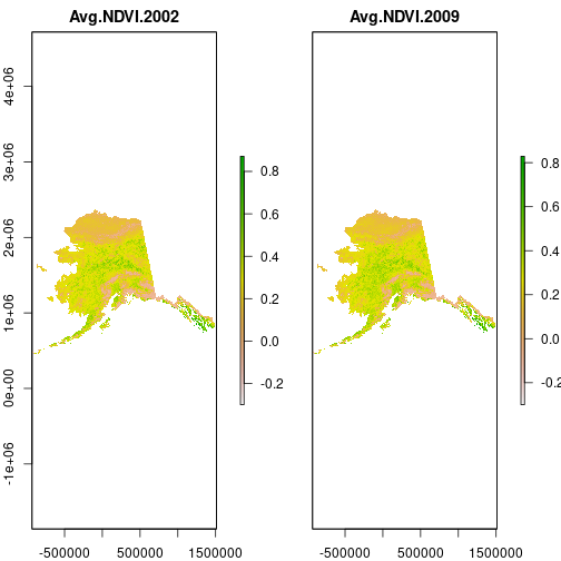
ndvi <- stack(ndvi_yrly)
names(ndvi) <- c(
  'Avg NDVI 2002',
  'Avg NDVI 2009')

Using the stack() function we create a raster stack and assign it to the ndvi object. We name each layer in the stack by using the names function. These will also be the titles for the plots.

> plot(ndvi)

The data source for the first layer is the first file in the list. Note that the CRS is missing: it is quite possible to stack files with different projections. They only have to share a common extent and resolution.

> # display metadata for the 1st raster in the ndvi stack
> raster(ndvi, 1)

class      : RasterLayer 
dimensions : 1951, 2441, 4762391  (nrow, ncol, ncell)
resolution : 1000.045, 999.9567  (x, y)
extent     : -930708.7, 1510401, 454027.3, 2404943  (xmin, xmax, ymin, ymax)
crs        : NA 
source     : r_ndvi_2001_2009_filling6__STA_year2_Amplitude0.tif 
names      : Avg.NDVI.2002 
values     : -0.3, 0.8713216  (min, max)

Set the CRS using the EPSG code 3338 for an Albers Equal Area projection of Alaska using the NAD38 datum.

crs(ndvi) <- '+init=epsg:3338'

> # display metadata for the ndvi stack
> raster(ndvi, 0)

class      : RasterLayer 
dimensions : 1951, 2441, 4762391  (nrow, ncol, ncell)
resolution : 1000.045, 999.9567  (x, y)
extent     : -930708.7, 1510401, 454027.3, 2404943  (xmin, xmax, ymin, ymax)
crs        : +proj=aea +lat_0=50 +lon_0=-154 +lat_1=55 +lat_2=65 +x_0=0 +y_0=0 +datum=NAD83 +units=m +no_defs 

The ndvi object only takes up a tiny amount of memory. The pixel values take up much more space on disk, as you can see in the file browser.

> print(object.size(ndvi),
+   units = 'KB',
+   standard = 'SI')

36.7 kB

Why so small? The ndvi object is only metadata and a pointer to where the pixel values are saved on disk.

> inMemory(ndvi)

[1] FALSE

Whereas read.csv() would load the named file into memory, the raster library handles files like a database where possible. The values can be accessed, to make those plots for example, but are not held in memory. This is the key to working with deep stacks of large rasters.

Wildfires in Alaska

Many and massive wildfires burned in Alaska and the Yukon between 2001 and 2009. Three large fires that burned during this period (their locations are in a shapefile) occurred within boreal forest areas of central Alaska.

scar <- st_read(
  'data/OVERLAY_ID_83_399_144_TEST_BURNT_83_144_399_reclassed',
  crs = 3338)

Reading layer `OVERLAY_ID_83_399_144_TEST_BURNT_83_144_399_reclassed' from data source `/nfs/public-data/training/OVERLAY_ID_83_399_144_TEST_BURNT_83_144_399_reclassed' 
  using driver `ESRI Shapefile'

Warning: st_crs<- : replacing crs does not reproject data; use st_transform for
that

Simple feature collection with 3 features and 2 fields
Geometry type: MULTIPOLYGON
Dimension:     XY
Bounding box:  xmin: 68336.13 ymin: 1772970 xmax: 219342.9 ymax: 1846967
Projected CRS: NAD83 / Alaska Albers

plot(ndvi[[1]])
plot(st_geometry(scar), add = TRUE)

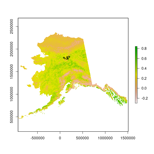
We read the OVERLAY_ID_83_399_144_TEST_BURNT_83_144_399_reclassed directory. This is a polygon shapefile containing the geometry of a wildfire in central Alaska. We assign the EPSG:3338 CRS for Alaska Albers when reading the shapefile. We plot the first raster layer in the ndvi stack and then plot an overlay of the wildfire using the polygon shapefile.

For faster processing in this lesson, crop the NDVI imagery to the smaller extent of the shapefile.

burn_bbox <- st_bbox(scar)
ndvi <- crop(ndvi, burn_bbox)

Using st_bbox() we find the bounding box of the wildfire scar polygons. We assign it to burn_bbox and crop the raster stack object ndvi to that extent.

> plot(ndvi[[1]], ext = burn_bbox)
> plot(st_geometry(scar), add = TRUE)

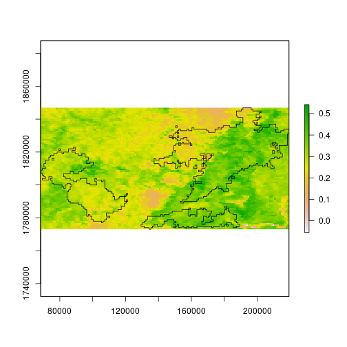
Notice, however, that the NDVI values are now stored in memory. That’s okay for this part of the lesson; we’ll see the alternative shortly.

> inMemory(ndvi)

[1] TRUE

Pixel Change

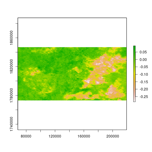
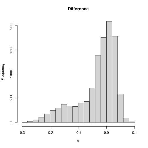
Use element-wise subtraction to give a difference raster, where negative values indicate a higher NDVI in 2002, or a decrease in NDVI from 2002 to 2009.

diff_ndvi <- ndvi[[2]] - ndvi[[1]]
names(diff_ndvi) <- 'Difference'

diff_ndvi is a raster object containing the difference between the NDVI values for 2002 and 2009 for each pixel.

> plot(diff_ndvi)

The histogram shows clearly that change in NDVI within this corner of Alaska clusters around two modes.

> hist(diff_ndvi)

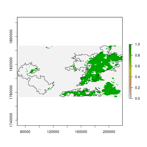
One way to “classify” pixels as potentially affected by wildfire is to threshold the difference. Pixels below -0.1 mostly belong to the smaller mode, and may represent impacts of wildfire.

> plot(diff_ndvi < -0.1)
> plot(st_geometry(scar), add = TRUE)

The threshold value could also be defined in terms of the variability among pixels.

Centering and scaling the pixel values requires computation of their mean and standard variation. The cellStats function efficiently applies a few common functions across large rasters, regardless of whether the values are in memory or on disk.

diff_ndvi_mean <-
  cellStats(diff_ndvi, 'mean')
diff_ndvi_sd <-
  cellStats(diff_ndvi, 'sd')

Mathematical operations with rasters and scalars work as expected; scalar values are repeated for each cell in the array.

The difference threshold of -0.1 appears roughly equivalent to a threshold of 1 standard deviation below zero.

In the following code block we standardize the NDVI difference by subtracting the mean we calculated earlier, and then dividing by the standard deviation.

diff_ndvi_stdz <-
  (diff_ndvi - diff_ndvi_mean) /
  diff_ndvi_sd
names(diff_ndvi_stdz) <- 'Std. Diff.'

> hist(diff_ndvi_stdz, breaks = 20)

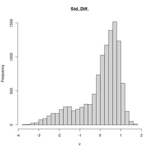
Standardizing the pixel values does not change the overall result.

> plot(diff_ndvi_stdz < -1)
> plot(st_geometry(scar), add = TRUE)

Raster Time Series

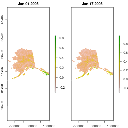
Take a closer look at NDVI using products covering 16-day periods in 2005. These images are stored as separate files on the disk, all having the same extent and resolution.

ndvi_16day <- Sys.glob(
  'data/NDVI_alaska_2005/*.tif')
ndvi <- stack(ndvi_16day)
crs(ndvi) <- '+init=epsg:3338'

The ndvi_16day object contains the names for all the .tif files in the data/NDVI_alaska_2005/ folder. We create a stack of rasters and assign a CRS.

Lacking other metadata, extract the date of each image from its filename.

dates <- as.Date(
  sub('alaska_NDVI_', '', names(ndvi)),
  '%Y_%m_%d')
names(ndvi) <- format(dates, '%b %d %Y')

All the raster images are stored in the ndvi stack object and their names start with alaska_NDVI_. names(ndvi) gives us all the names of the rasters in the stack. First we use sub() to replace alaska_NDVI_ with an empty string, which gives us just the dates. We then format the dates, and assign them back as the names for the rasters in the stack. In this case, we are formatting the dates like so: '%b %d %Y', where %b is the month, %d the day, and %Y the year.

> plot(subset(ndvi, 1:2))

Raster Bricks

A RasterBrick representation of tightly integrated raster layers, such as a time series of remote sensing data from sequential overflights, has advantages for speed but limitations on flexibility.

A RasterStack is more flexible because it can mix values stored on disk with those in memory. Adding a layer of in-memory values to a RasterBrick causes the entire brick to be loaded into memory, which may not be possible given the available memory.

RasterBrick can be created from a RasterStack

For training purposes, again crop the NDVI data to the bounding box of the wildfires shapefile. But this time, avoid reading the values into memory.

ndvi <- crop(ndvi, burn_bbox,
  filename = file.path(out, 'crop_alaska_ndvi.grd'),
  overwrite = TRUE)

Notice that crop creates a RasterBrick. In fact, we have been working with a RasterBrick in memory since first using crop.

> ndvi

class      : RasterBrick 
dimensions : 74, 151, 11174, 23  (nrow, ncol, ncell, nlayers)
resolution : 1000.045, 999.9566  (x, y)
extent     : 68336.16, 219342.9, 1772970, 1846967  (xmin, xmax, ymin, ymax)
crs        : +proj=aea +lat_0=50 +lon_0=-154 +lat_1=55 +lat_2=65 +x_0=0 +y_0=0 +datum=NAD83 +units=m +no_defs 
source     : crop_alaska_ndvi.grd 
names      : Jan.01.2005, Jan.17.2005, Feb.02.2005, Feb.18.2005, Mar.06.2005, Mar.22.2005, Apr.07.2005, Apr.23.2005, May.09.2005, May.25.2005, Jun.10.2005, Jun.26.2005, Jul.12.2005, Jul.28.2005, Aug.13.2005, ... 
min values :    -0.19518,    -0.20000,    -0.19900,    -0.18050,    -0.12120,    -0.09540,    -0.03910,    -0.11290,    -0.09390,    -0.15520,    -0.18400,    -0.16780,    -0.18000,    -0.17200,    -0.18600, ... 
max values :   0.3337000,   0.3633000,   0.4949000,   0.3514000,   0.4898000,   0.7274000,   0.6268000,   0.5879000,   0.9076000,   0.9190000,   0.8807000,   0.9625000,   0.8810000,   0.9244000,   0.9493000, ... 

So Much Data

The immediate challenge is trying to represent the data in ways we can explore and interpret the characteristics of wildfire visible by remote sensing.

> animate(ndvi, pause = 0.5, n = 1)

Pixel Time Series

Verify that something happened very abruptly (fire!?) by plotting the time series at pixels corresponding to locations with dramatic NDVI variation in the layer from Aug 13, 2005.

idx <- match('Aug.13.2005', names(ndvi))
plot(ndvi[[idx]])

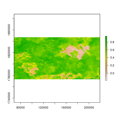
match() returns the index of the layer in ndvi named 'Aug.13.2005'.

> pixel <- click(ndvi[[idx]], cell = TRUE)
> pixel

click() gives us the ability to click on the plot map and get pixel values for a cell. After clicking on the map, you will see the cell number and value for that cell is printed on the console. Press the esc key to exit the pixel clicker.

“Hard code” these pixel values into your worksheet.

pixel <- c(2813, 3720, 2823, 4195, 9910)
scar_pixel <- data.frame(
  Date = rep(dates, each = length(pixel)),
  cell = rep(pixel, length(dates)),
  Type = 'burn scar?',
  NDVI = c(ndvi[pixel]))

We create a scar_pixel dataframe for the burn scar. rep() repeats the dates each times (the number of pixels). pixel is repeated for each of the dates.

Repeat the selection with click for “normal” looking pixels.

pixel <- c(1710, 4736, 7374, 1957, 750)
normal_pixel <- data.frame(
  Date = rep(dates, each = length(pixel)),
  cell = rep(pixel, length(dates)),
  Type = 'normal',
  NDVI = c(ndvi[pixel]))

Join your haphazard samples together for comparison as time series.

pixel <- rbind(normal_pixel, scar_pixel)
ggplot(pixel,
       aes(x = Date, y = NDVI,
           group = cell, col = Type)) +
  geom_line()

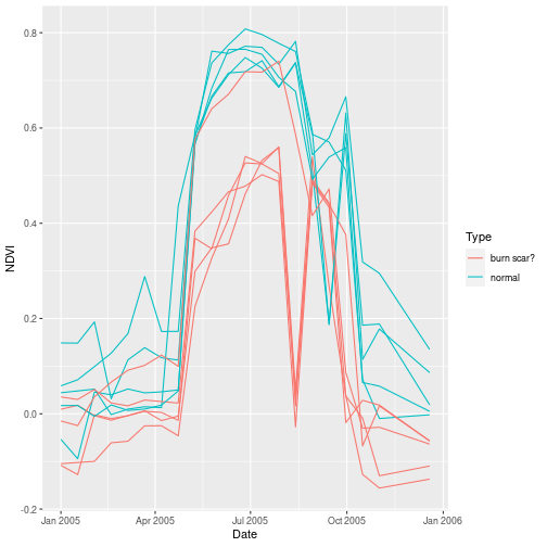
Combine the two dataframes we created to a single one and plot with ggplot(). We can see a significant difference in August between a possible burn scar and what the area normally looks like.

Zonal Averages

We cannot very well analyze the time series for every pixel, so we have to reduce the dimensionality of the data. One way is to summarize it by “zones” defined by another spatial data source.

> ?zonal

Currently we have raster data (ndvi) and vector data (scar). In order to aggregate by polygon, we have to join these two datasets. There are two approaches. 1) Treat the raster data as POINT geometries in a table and perform a spatial join to the table with POLYGON geometries. 2) Turn the polygons into a raster and summarize the raster masked for each polygon. Let’s pursue option 2.

Let’s convert out scar shapefile to raster with the rasterize function.

# Rasterize polygon shapefile.
scar_geom <-
  as(st_geometry(scar), 'Spatial')
scar_zone <- rasterize(scar_geom, ndvi,
  background = 0,
  filename = 'outputs_raster_ts/scar.grd',
  overwrite = TRUE)

crs(scar_zone) <- '+init=epsg:3338'
scar_zone <- crop(scar_zone, ndvi)

Using as() we coerce the scar shapefile as an object of the ‘Spatial’ class. We then use rasterize() to create a RasterLayer object for the shapefile. Then we crop the raster to the same extent as ndvi.

The zonal function calculates fun (here, mean) over each zone.

scar_ndvi <-
  zonal(ndvi, scar_zone, "mean")

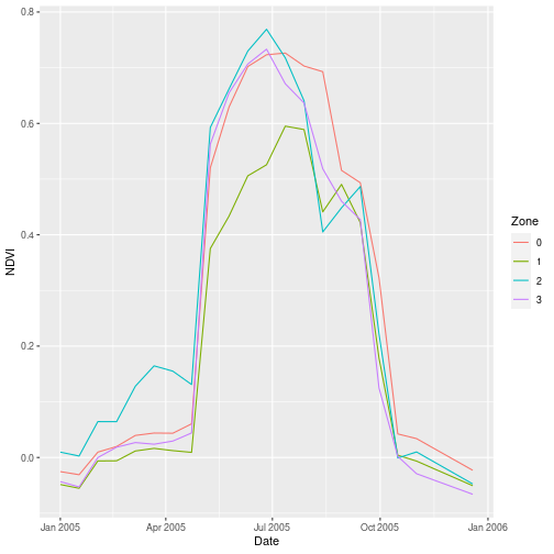
Rearrange the data for visualization as a time series.

zone <- factor(scar_ndvi[, 1])
scar_ndvi <- scar_ndvi[, -1]
scar_zone <- data.frame(
  Date = rep(dates, each = nrow(scar_ndvi)),
  Zone = rep(zone, length(dates)),
  NDVI = c(scar_ndvi))

Here we convert the zone category labels to a factor variable, then manually reshape the data from wide form to long form, with one column for the date, one for the zone category, and one for the mean NDVI value for that category.

What appears to be the most pronounced signal in this view is an early loss of greenness compared to the background NDVI (Zone 0).

> ggplot(scar_zone,
+        aes(x = Date, y = NDVI,
+            col = Zone)) +
+   geom_line()

Zonal Statistics

• provide a very clean reduction of raster time-series for easy visualization
• require pre-defined zones!

Eliminating Time

Because changes to NDVI at each pixel follow a similar pattern over the course of a year, the slices are highly correlated. Consider representing the NDVI values as a simple matrix with

• each time slice as a variable
• each pixel as an observation

Principal component analysis (PCA), is an image classification technique. It is a technique for reducing dimensionality of a dataset based on correlation between variables. The method proceeds either by eigenvalue decomposition of a covariance matrix or singular-value decomposition of the entire dataset. Principal components are the distinctive or peculiar features of an image.

To perform PCA on raster data, it’s efficient to use specialized tools that calculate a covariance matrix without reading in that big data matrix.

ndvi_lS <- layerStats(
  ndvi, 'cov', na.rm = TRUE)
ndvi_mean <- ndvi_lS[['mean']]
ndvi_cov <- ndvi_lS[['covariance']]
ndvi_cor <- cov2cor(ndvi_cov)

Here, we use layerStats to calculate the covariance between each pair of layers (dates) in our NDVI brick, and the mean of each date. layerStats calculates summary statistics across multiple layers of a RasterStack or RasterBrick, analogous to how cellStats calculates summary statistics for each layer separately. After calculating the summary statistics we extract each one to a separate object and then scale the covariance matrix using cov2cor.

The layerStats function only evaluates standard statistical summaries. The calc function, however, can apply user-defined functions over or across raster layers.

ndvi_std <- sqrt(diag(ndvi_cov))
ndvi_stdz <- calc(ndvi,
  function(x) (x - ndvi_mean) / ndvi_std,
  filename = file.path(out, 'ndvi_stdz.grd'),
  overwrite = TRUE)

Here we find the standard deviation of each NDVI time slice by pulling out the diagonal of the covariance matrix with diag(), which contains the variance of each time slice, then taking the square root of the variance. Next, inside calc(), we define a function inline to standardize a value by subtracting the mean then dividing by the standard deviation, then apply it to each pixel in each layer of ndvi. We use filename to write the output directly to disk.

Standardizing the data removes the large seasonal swing, but not the correlation between “variables,” i.e., between pixels in different time slices. Only the correlation matters for PCA.

> animate(ndvi_stdz, pause = 0.5, n = 1)

Now, we use princomp to calculate the principal components of the NDVI correlations, which is just a 23-by-23 matrix of pairwise correlations between the 23 time slices. The plot method of the output shows the variance among pixels, not at each time slice, but on each principal component.

pca <- princomp(covmat = ndvi_cor)
plot(pca)

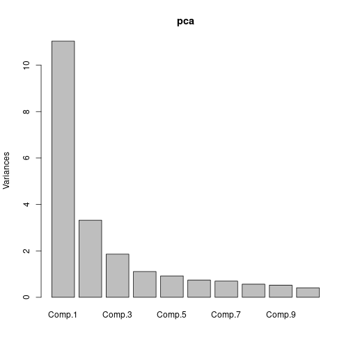
The bar plot of eigenvalues expressed in percentage plotted above gives us the information retained in each principal component (PC). Notice that the last PCs eigenvalues are small and less significant, this is where dimensionality reduction comes into play. If we chose to keep the first four relevant components that retain most of the information then the final data can be reduced to 4 PCs without loosing much information.

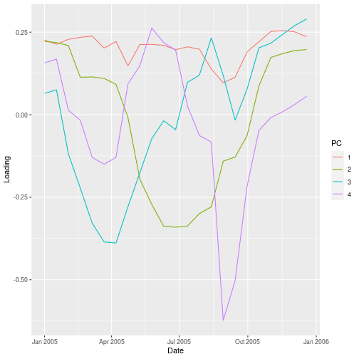
Principal component “loadings” correspond to the weight each time slice contributes to each component.

npc <- 4
loading <- data.frame(
  Date = rep(dates, npc), 
  PC = factor(
    rep(1:npc, each = length(dates))
  ),
  Loading = c(pca$loadings[, 1:npc])
)

Here we manually reshape the output of princomp into a data frame for plotting.

The first principal component is a more-or-less equally weighted combination of all time slices, like an average.

In contrast, components 2 through 4 show trends over time. PC2 has a broad downward trend centered around July 2005, while PC3 has a sharp downward trend centered around April 2005.

ggplot(loading,
       aes(x = Date, y = Loading,
           col = PC)) +
  geom_line()

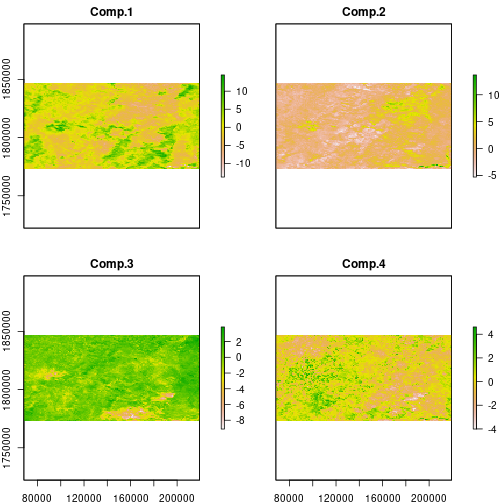
The principal component scores are projections of the NDVI values at each time point onto the components. Memory limitation may foil a straightforward attempt at this calculation, but the raster package predict wrapper carries the princomp predict method through to the time series for each pixel.

pca$center <- pca$scale * 0
ndvi_scores <- predict(
  ndvi_stdz, pca,
  index = 1:npc,
  filename = file.path(out, 'ndvi_scores.grd'),
  overwrite = TRUE)
plot(ndvi_scores)

A complication in here is that the pca object does not know how the original data were centered, because we didn’t give it the original data. The predict function will behave as if we performed PCA on ndvi_stdz[] if we set the centering vector to zeros. We specify index = 1:npc to restrict the prediction to the first four principal component axes. This returns a standardized value for each pixel on each of the four axes.

The first several principal components account for most of the variance in the data, so approximate the NDVI time series by “un-projecting” the scores.

Mathematically, the calculation for this approximation at each time slice, \(\mathbf{X_t}\), is a linear combination of each score “map”, \(\mathbf{T}_i\), with time-varying loadings, \(W_{i,t}\).

The flexible overlay function allows you to pass a custom function for pixel-wise calculations on one or more of the main raster objects.

ndvi_dev <- overlay(
  ndvi_stdz, ndvi_scores,
  fun = function(x, y) {
    x - y %*% t(pca$loadings[, 1:npc])
  },
  filename = file.path(out, 'ndvi_dev.grd'),
  overwrite = TRUE)
names(ndvi_dev) <- names(ndvi)

Here we define a function fun that takes two arguments, x and y. Those are the first two arguments we pass to overlay. The overlay function then “overlays” raster brick x, the standardized NDVI time series with 23 layers, on raster brick y, the first 4 PCA scores for that time series, and applies fun to each pixel of those two raster bricks. fun performs matrix multiplication of one pixel of y with the first 4 PCA loadings and then subtracts the result from x, resulting in the difference between the observed standardized pixel values and the values predicted by the principal components.

Verify that the deviations just calculated are never very large, (that is, the PCA predicts the true values fairly well), then try the same approximation using even fewer principal components.

> animate(ndvi_dev, pause = 0.5, n = 1)

Based on the time variation in the loadings for principal components 2 and 3, as we saw in the graph of loadings versus time we made earlier, we might guess that they correspond to one longer-term and one shorter-term departure from the seasonal NDVI variation within this extent.

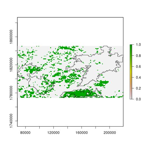
plot(
  ndvi_scores[[2]] < -2 |
  ndvi_scores[[3]] < -2)
plot(st_geometry(scar), add = TRUE)

Summary

The RasterBrick objects created by the brick function, or sometimes as the result of calculations on a RasterStack, are built for many layers of large rasters. Key principles for efficient analysis of raster time series include:

• consolidate RasterStacks to RasterBricks for faster computation
• provide filename arguments to keep objects on disk
• use layerStats to get a covariance matrix for Principal Component Analysis (PCA)
• use calc and overlay to call custom functions

Takeaways:

• The raster package has two classes for multi-layer data the RasterStacks and the RasterBrik.
• RasterBrik can only be linked to a single (multi-layer) file.
• RasterStack can be formed from separate files and/or from a few layers from a single file.
• PCA is a dimensionality-reduction method used to reduce the dimensionality of a large data set improving algorithm and analysis performance and speed.