Remote Sensing & Classification
Hurricane Inundation
Note: This lesson is in beta status! It may have issues that have not been addressed.
Handouts for this lesson need to be saved on your computer. Download and unzip this material into the directory (a.k.a. folder) where you plan to work.
Remote Sensing allows for fast generation of maps before and after events. In this exercise, you will map flooding using machine learning methods and MODIS reflectance data (MOD09). Hurricanes can strongly impact vegetation and human settlements. Hurricane Rita made landfall on September 24, 2005 in Louisiana near the border with Texas. In addition to the rainfall, the hurricane was accompanied by a storm surge that generated flooding and a large amount of damage to ground infrastructure and vegetation. As a geospatial analyst, you will experiment with different classifiers for rapid mapping and examine their performance with training and testing data. All work must be repeatable and documented in a scripting environment to be shared with your team.
Inputs
- FEMA flood map (stored as vector data)
- MOD09 reflectance image after Hurricane Rita
- Vector polygons of ground truth (for training and testing classifiers)
- NLCD 2006 land cover aggregated at 1km
Outputs
- classified map using rpart classifier
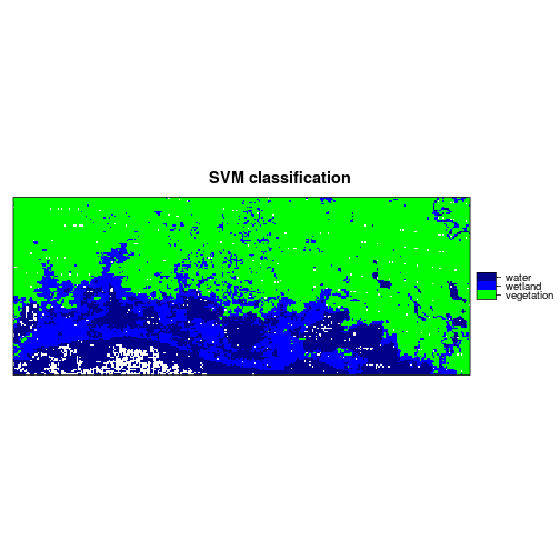
- classified map using svm classifier
- confusion matrices and overall accuracies by classifiers
Tools/Functions
- raster::brick
- raster::writeRaster
- sf::st_read
- raster::subset
- raster::extract
- raster::predict
- raster algebra: “*”,” /”,”+”,”-“
- rasterVis::levelplot
- rasterVis::histogram
Part I: Read and map flooding from RITA hurricane
Explore the datasets provided. Use ground truth vector datasets and extract values for pixels for the raster stack containing the original MOD09 bands and indices. Visualize ground truth pixels in feature space and using boxplots.
Products:
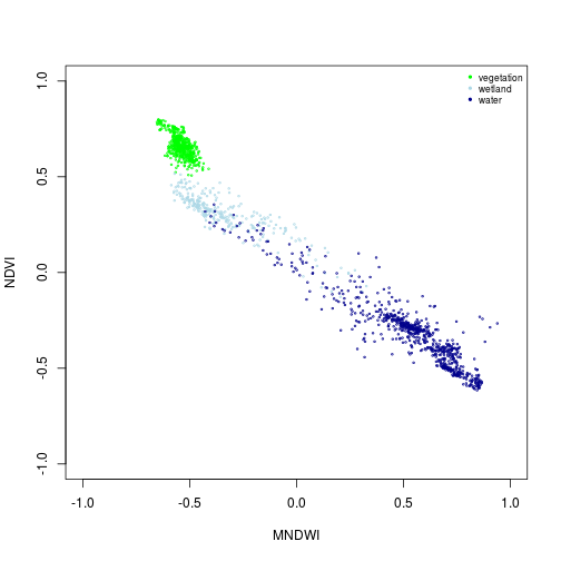
- Scatterplot in feature space with the three ground classes.
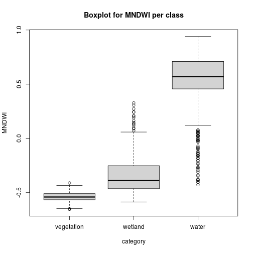
- Boxplots of values for MNDWI indices.
Part II: Split data into training and testing datasets
Assessment of classifications require splitting of the ground truth data into training and testing samples. The training data is used in the fitting of the model while the testing dataset is used accuracy assessment. Using the data provided randomly select 30% ground truth data for testing.
Products:
- Training and testing datasets at 30%. Save these into shapefiles.
Be able to answer the following question:
- What is the frequency of observations in each class for training and testing data?
Part III: Generate classification using classification tree (CART) and support vector machine (SVM)
You will use MOD09 reflectance bands to generate a classification of three classes (“vegetation”, “wetland”, “water”). Fit a model with the training data for each method and generate a classification on a raster using the “predict” command.
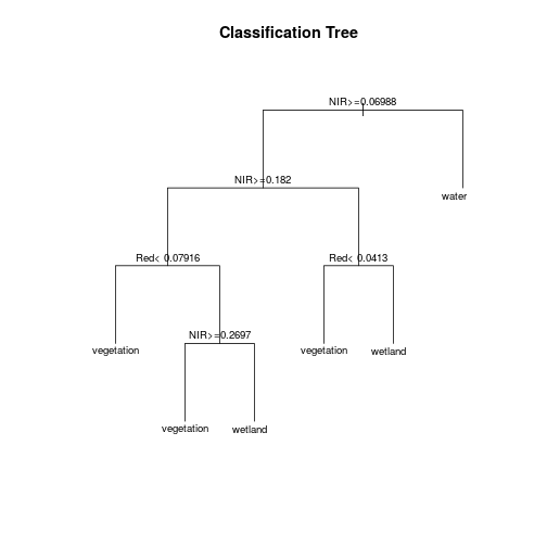
RPART: It is based on CART and generates classification by splitting data points into branches successively and generating classified pixels. The rules generated from the tree can then be applied to the full raster image to produce a prediction.
SVM: Support Vector Machine generate hyperplanes that maximize separabiltiy between classes.These hyperplanes boundaries are used in the classification process and generate predictions.
Products:
- Model object for rpart with a predicted raster.
- Model object for svm with a predicted raster
Part IV: Assessment and comparison of model performance
To validate the model, we use the testing data and generate new predictions for rpart and SVM. We compare the predictions with the original testing information.
Overall accuracy: total number of correctly classified pixels for all classes combined over the total number of pixels.
Producer accuracy: is the fraction of correctly classified pixels with regard to all pixels of the ground truth class.
Products:
- Overall accuracy and producer accuracy metrics.
- Confusion matrix for rpart and SVM.
Be able to answer the following question:
- What classifier had the best overall accuracy?
Using the analyses performed above, and datasets provided answer to the following questions:
- Modify the splitting of training and testing by using 40% and then 50% for testing. Compare predicted maps with previous results.
- Generate confusion matrices for 40% and 50% testing.
- Generate a classification prediction using randomForest and compare it to svm and rpart with 30% holdout.
Set up arguments and parameters
in_dir <- "data"

out_dir_suffix <- "rsc_lesson"
out_dir <- paste("output_", out_dir_suffix, sep = "")
dir.create(out_dir, showWarnings = FALSE)
Regional coordinate reference system taken from: http://spatialreference.org/ref/epsg/nad83-texas-state-mapping-system/proj4/
CRS_reg <- "+proj=lcc +lat_1=27.41666666666667 +lat_2=34.91666666666666 +lat_0=31.16666666666667 +lon_0=-100 +x_0=1000000 +y_0=1000000 +ellps=GRS80 +datum=NAD83 +units=m +no_defs"

file_format <- ".tif"

NA_flag_val <- -9999

out_suffix <- "raster_classification" # output suffix for the files and output folder
Define input data file names
infile_RITA_reflectance_date2 <- "mosaiced_MOD09A1_A2005273__006_reflectance_masked_RITA_reg_1km.tif"

infile_reg_outline <- "new_strata_rita_10282017" # Region outline and FEMA zones

infile_modis_bands_information <- "df_modis_band_info.txt" # MOD09 bands information.

nlcd_2006_filename <- "nlcd_2006_RITA.tif" # NLCD2006 Land cover data aggregated at ~ 1km.
Part I: Read and map flooding from RITA hurricane
Display and explore the data
MOD09 raster image after hurricane Rita.
r_after <- brick(file.path(in_dir, infile_RITA_reflectance_date2))
> head(r_after)
mosaiced_MOD09A1_A2005273__006_reflectance_masked_RITA_reg_1km.1
[1,] 0.04558113
[2,] 0.04460510
[3,] 0.04348749
[4,] 0.04507260
[5,] 0.04715690
[6,] 0.03485106
[7,] 0.03807684
[8,] 0.04214056
[9,] 0.04512509
[10,] 0.04687950
[11,] 0.04639116
[12,] 0.04591873
[13,] 0.04590000
[14,] 0.05590000
[15,] 0.05367381
[16,] 0.05220000
[17,] 0.05146399
[18,] 0.04496353
[19,] 0.04380151
[20,] 0.06080000
mosaiced_MOD09A1_A2005273__006_reflectance_masked_RITA_reg_1km.2
[1,] 0.3027903
[2,] 0.3043112
[3,] 0.2998908
[4,] 0.3017146
[5,] 0.3239896
[6,] 0.2683164
[7,] 0.2991171
[8,] 0.3176138
[9,] 0.3125040
[10,] 0.2979249
[11,] 0.3101786
[12,] 0.3076983
[13,] 0.3076000
[14,] 0.2953000
[15,] 0.3113045
[16,] 0.3219000
[17,] 0.3242094
[18,] 0.3254988
[19,] 0.3138167
[20,] 0.3098000
mosaiced_MOD09A1_A2005273__006_reflectance_masked_RITA_reg_1km.3
[1,] 0.02379627
[2,] 0.02354558
[3,] 0.02374887
[4,] 0.02426019
[5,] 0.02511090
[6,] 0.01941371
[7,] 0.02170737
[8,] 0.02348050
[9,] 0.02387191
[10,] 0.02560453
[11,] 0.02765067
[12,] 0.02635150
[13,] 0.02630000
[14,] 0.03030000
[15,] 0.02999916
[16,] 0.02980000
[17,] 0.02756310
[18,] 0.02447605
[19,] 0.02306678
[20,] 0.03420000
mosaiced_MOD09A1_A2005273__006_reflectance_masked_RITA_reg_1km.4
[1,] 0.05476730
[2,] 0.05586702
[3,] 0.05381133
[4,] 0.05503851
[5,] 0.05962222
[6,] 0.04450204
[7,] 0.04927124
[8,] 0.05364913
[9,] 0.05487191
[10,] 0.05564768
[11,] 0.05650510
[12,] 0.05544214
[13,] 0.05540000
[14,] 0.05870000
[15,] 0.06014401
[16,] 0.06110000
[17,] 0.06231735
[18,] 0.05556127
[19,] 0.05338556
[20,] 0.06660000
mosaiced_MOD09A1_A2005273__006_reflectance_masked_RITA_reg_1km.5
[1,] 0.3318335
[2,] 0.3138186
[3,] 0.3123330
[4,] 0.3193893
[5,] 0.3417773
[6,] 0.2855803
[7,] 0.3055280
[8,] 0.3266653
[9,] 0.3330796
[10,] 0.3139284
[11,] 0.3352741
[12,] 0.3151959
[13,] 0.3144000
[14,] 0.3485000
[15,] 0.3409190
[16,] 0.3359000
[17,] 0.3346323
[18,] 0.3365578
[19,] 0.3272987
[20,] 0.3235000
mosaiced_MOD09A1_A2005273__006_reflectance_masked_RITA_reg_1km.6
[1,] 0.1902746
[2,] 0.1842244
[3,] 0.1855501
[4,] 0.1913280
[5,] 0.1930779
[6,] 0.1609111
[7,] 0.1696934
[8,] 0.1781321
[9,] 0.1907084
[10,] 0.1913635
[11,] 0.1840112
[12,] 0.1886174
[13,] 0.1888000
[14,] 0.2295000
[15,] 0.2199936
[16,] 0.2137000
[17,] 0.2036836
[18,] 0.1829669
[19,] 0.1818172
[20,] 0.2122000
mosaiced_MOD09A1_A2005273__006_reflectance_masked_RITA_reg_1km.7
[1,] 0.07314926
[2,] 0.06792310
[3,] 0.07248760
[4,] 0.07654412
[5,] 0.07032830
[6,] 0.05962812
[7,] 0.06153552
[8,] 0.06410249
[9,] 0.07345820
[10,] 0.07704768
[11,] 0.06562383
[12,] 0.07223780
[13,] 0.07250001
[14,] 0.10140000
[15,] 0.09135209
[16,] 0.08470000
[17,] 0.07624704
[18,] 0.06806806
[19,] 0.06944025
[20,] 0.09370000
> inMemory(r_after) # check if raster in memory
[1] FALSE
Read band information since it is more informative.
df_modis_band_info <- read.table(file.path(in_dir, infile_modis_bands_information),
                                 sep=",", stringsAsFactors = F)
> df_modis_band_info
  band_name band_number start_wlength end_wlength
1       Red           3           620         670
2       NIR           4           841         876
3      Blue           1           459         479
4     Green           2           545         565
5     SWIR1           5          1230        1250
6     SWIR2           6          1628        1652
7     SWIR3           7          2105        2155
names(r_after) <- df_modis_band_info$band_name
> names(r_after)
[1] "Red" "NIR" "Blue" "Green" "SWIR1" "SWIR2" "SWIR3"
Define bands of interest: Use subset instead of $ if you want to wrap code into function
raft_gr <- subset(r_after, "Green")
raft_SWIR <- subset(r_after, "SWIR2")
raft_NIR <- subset(r_after, "NIR")
raft_rd <- subset(r_after, "Red")
Manipulate bands of interest
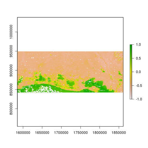
r_after_MNDWI <- (raft_gr - raft_SWIR) / (raft_gr + raft_SWIR)

plot(r_after_MNDWI, zlim = c(-1,1))
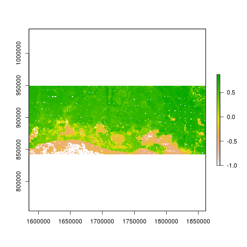
r_after_NDVI <- (raft_NIR - raft_rd) / (raft_NIR + raft_rd)

plot(r_after_NDVI)
> inMemory(r_after_MNDWI) # check if raster in memory
[1] TRUE
> inMemory(r_after_NDVI)
[1] TRUE
Write out rasters
> dataType(r_after_NDVI)
[1] "FLT4S"
data_type_str <- dataType(r_after_NDVI)

NAvalue(r_after_MNDWI) <- NA_flag_val # set NA value
out_filename_mn <- file.path(out_dir, paste0("mndwi_post_Rita","_", out_suffix, file_format))
writeRaster(r_after_MNDWI, filename = out_filename_mn, datatype = data_type_str,
            overwrite = T)

NAvalue(r_after_NDVI) <- NA_flag_val
out_filename_nd <- file.path(out_dir, paste0("ndvi_post_Rita","_", out_suffix, file_format))
writeRaster(r_after_NDVI, filename = out_filename_nd, datatype = data_type_str,
            overwrite = T)
Remove rasters from memory
rm(r_after_MNDWI)
rm(r_after_NDVI)
Can view the .tif images written out in photo viewer.
Read in rasters
r_after_MNDWI <- raster(out_filename_mn)
r_after_NDVI <- raster(out_filename_nd)
> inMemory(r_after_MNDWI) ; inMemory(r_after_NDVI)
[1] FALSE
[1] FALSE
Groundtruthing data
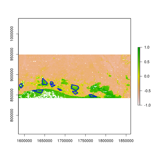
Three levels of flooding (water content) determined via external grountruthing. Class 1: vegetation and other (small water fraction) Class 2: Flooded vegetation Class 3: Flooded area, or water (lake etc)
Read in a polygon for each class:
class1_data_sf <- st_read(file.path(in_dir, "class1_sites"))
Reading layer `class1_sites' from data source `/nfs/public-data/training/class1_sites' using driver `ESRI Shapefile'
Simple feature collection with 6 features and 2 fields
geometry type:  POLYGON
dimension:      XY
bbox:           xmin: 1588619 ymin: 859495.9 xmax: 1830803 ymax: 941484.1
CRS:            NA
class2_data_sf <- st_read(file.path(in_dir, "class2_sites"))
Reading layer `class2_sites' from data source `/nfs/public-data/training/class2_sites' using driver `ESRI Shapefile'
Simple feature collection with 8 features and 2 fields
geometry type:  MULTIPOLYGON
dimension:      XY
bbox:           xmin: 1605433 ymin: 848843.8 xmax: 1794265 ymax: 884027.8
CRS:            NA
class3_data_sf <- st_read(file.path(in_dir, "class3_sites"))
Reading layer `class3_sites' from data source `/nfs/public-data/training/class3_sites' using driver `ESRI Shapefile'
Simple feature collection with 9 features and 2 fields
geometry type:  POLYGON
dimension:      XY
bbox:           xmin: 1587649 ymin: 845271.3 xmax: 1777404 ymax: 891073.1
CRS:            NA
> class1_data_sf
Simple feature collection with 6 features and 2 fields
geometry type:  POLYGON
dimension:      XY
bbox:           xmin: 1588619 ymin: 859495.9 xmax: 1830803 ymax: 941484.1
CRS:            NA
  record_ID class_ID                       geometry
1         1        1 POLYGON ((1610283 929863.7,...
2         2        1 POLYGON ((1755141 900167.2,...
3         3        1 POLYGON ((1688209 924699.1,...
4         4        1 POLYGON ((1821103 866597.2,...
5         5        1 POLYGON ((1806876 941161.3,...
6         6        1 POLYGON ((1588619 899198.8,...
> plot(r_after_MNDWI, zlim=c(-1,1))
> plot(class3_data_sf["class_ID"], add = TRUE, color = NA, border = "blue", lwd = 3)
Combine polygons; note they should be in the same projection system.
class_data_sf <- rbind(class1_data_sf, class2_data_sf, class3_data_sf)

class_data_sf$poly_ID <- 1:nrow(class_data_sf) # unique ID for each polygon
23 different polygons used as ground truth data.
> nrow(class_data_sf)
[1] 23
Make new rasters and raster stack.
r_x <- init(r_after, "x") # initializes a raster with coordinates x
r_y <- init(r_after, "y") # initializes a raster with coordiates y

r_stack <- stack(r_x, r_y, r_after, r_after_NDVI, r_after_MNDWI)
names(r_stack) <- c("x", "y", "Red", "NIR", "Blue", "Green", "SWIR1", "SWIR2", "SWIR3", "NDVI", "MNDWI")
> str(r_stack, max.level = 2)
Formal class 'RasterStack' [package "raster"] with 11 slots
  ..@ filename: chr ""
  ..@ layers  :List of 11
  ..@ title   : chr(0)
  ..@ extent  :Formal class 'Extent' [package "raster"] with 4 slots
  ..@ rotated : logi FALSE
  ..@ rotation:Formal class '.Rotation' [package "raster"] with 2 slots
  ..@ ncols   : int 298
  ..@ nrows   : int 116
  ..@ crs     :Formal class 'CRS' [package "sp"] with 1 slot
  ..@ history : list()
  ..@ z       : list()
pixels_extracted_df <- extract(r_stack, class_data_sf, df=T)
> dim(pixels_extracted_df)
[1] 1547 12
We have 1547 pixels extracted.
Sometimes useful to store data as a csv: have to remove geometry column.
class_data_df <- class_data_sf
st_geometry(class_data_df) <- NULL # This will coerce the sf object into a data.frame by removing the geometry
Make the dataframe used for classification.
pixels_df <- merge(pixels_extracted_df, class_data_df, by.x="ID", by.y="poly_ID")
> head(pixels_df)
  ID       x        y        Red       NIR       Blue      Green     SWIR1
1  1 1615340 936279.2 0.05304649 0.3035397 0.02652384 0.05662384 0.3101271
2  1 1614413 935352.5 0.05782417 0.3295924 0.02751791 0.06305390 0.3453724
3  1 1615340 935352.5 0.05735013 0.3037102 0.02596963 0.05654212 0.3176476
4  1 1616266 935352.5 0.05805403 0.3081988 0.02711912 0.05750944 0.3229090
5  1 1617193 935352.5 0.04147716 0.3058677 0.01839499 0.05076184 0.3003513
6  1 1618120 935352.5 0.04209801 0.3089238 0.01832494 0.05200353 0.2943777
      SWIR2      SWIR3      NDVI      MNDWI record_ID class_ID
1 0.1936452 0.07864757 0.7024759 -0.5474963         1        1
2 0.2102322 0.08679578 0.7014884 -0.5385503         1        1
3 0.2073480 0.08732812 0.6823238 -0.5714722         1        1
4 0.2079238 0.08741243 0.6829839 -0.5666749         1        1
5 0.1692552 0.06590501 0.7611759 -0.5385644         1        1
6 0.1697936 0.06790353 0.7601402 -0.5310712         1        1
table(pixels_df$class_ID) # count by class of pixels ground truth data
  1   2   3
508 285 754
Examining data used for the classification
Define geographic range.
x_range <- range(pixels_df$Green, na.rm=T)
y_range <- range(pixels_df$NIR, na.rm=T)
Let’s use a palette that reflects flooding or level of water.
col_palette <- c("green", "lightblue", "darkblue")
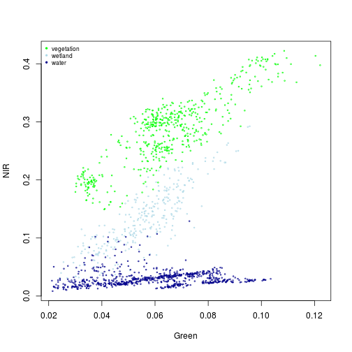
Many ways of looking at these data:
> plot(NIR~Green, xlim=x_range, ylim=y_range, cex=0.3, col=col_palette[1], subset(pixels_df, class_ID==1))
> points(NIR~Green, col=col_palette[2], cex=0.3, subset(pixels_df, class_ID==2))
> points(NIR~Green, col=col_palette[3], cex=0.3, subset(pixels_df, class_ID==3))
> names_vals <- c("vegetation","wetland","water")
> legend("topleft", legend=names_vals,
+        pt.cex=0.7, cex=0.7, col=col_palette,
+        pch=20, # add circle symbol to line
+        bty="n")
plot(NDVI ~ MNDWI, xlim=c(-1,1), ylim=c(-1,1), cex=0.3, col=col_palette[1], subset(pixels_df, class_ID==1))
points(NDVI ~ MNDWI, cex=0.3, col=col_palette[2], subset(pixels_df, class_ID==2))
points(NDVI ~ MNDWI, cex=0.3, col=col_palette[3], subset(pixels_df, class_ID==3))
names_vals <- c("vegetation","wetland","water")
legend("topright", legend=names_vals,
       pt.cex=0.7,cex=0.7, col=col_palette,
       pch=20, # add circle symbol to line
       bty="n")
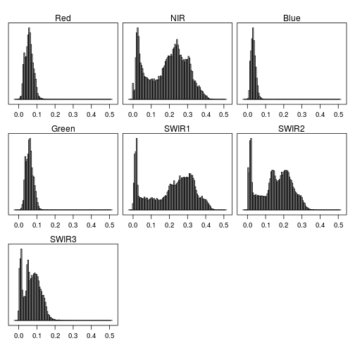
rasterVis::histogram(r_after)
pixels_df$class_ID <- factor(pixels_df$class_ID, levels = c(1,2,3), labels = names_vals)

boxplot(MNDWI~class_ID, pixels_df, xlab="category",
        main="Boxplot for MNDWI per class")
Part II: Split data into training and testing datasets
Let’s keep 30% of data for testing for each class, and set a fixed seed for reproducibility.
set.seed(100)
prop <- 0.3
table(pixels_df$class_ID)
vegetation    wetland      water
       508        285        754
list_data_df <- vector("list", length=3)
level_labels <- names_vals

for(i in 1:3){
  data_df <- subset(pixels_df, class_ID==level_labels[i])
  data_df$pix_id <- 1:nrow(data_df)
  indices <- as.vector(createDataPartition(data_df$pix_id, p=(1-prop), list=F))
  data_df$training <- as.numeric(data_df$pix_id %in% indices)
  list_data_df[[i]] <- data_df
}

data_df <- do.call(rbind, list_data_df)
> dim(data_df)
[1] 1547 16
> head(data_df)
  ID       x        y        Red       NIR       Blue      Green     SWIR1
1  1 1615340 936279.2 0.05304649 0.3035397 0.02652384 0.05662384 0.3101271
2  1 1614413 935352.5 0.05782417 0.3295924 0.02751791 0.06305390 0.3453724
3  1 1615340 935352.5 0.05735013 0.3037102 0.02596963 0.05654212 0.3176476
4  1 1616266 935352.5 0.05805403 0.3081988 0.02711912 0.05750944 0.3229090
5  1 1617193 935352.5 0.04147716 0.3058677 0.01839499 0.05076184 0.3003513
6  1 1618120 935352.5 0.04209801 0.3089238 0.01832494 0.05200353 0.2943777
      SWIR2      SWIR3      NDVI      MNDWI record_ID   class_ID pix_id
1 0.1936452 0.07864757 0.7024759 -0.5474963         1 vegetation      1
2 0.2102322 0.08679578 0.7014884 -0.5385503         1 vegetation      2
3 0.2073480 0.08732812 0.6823238 -0.5714722         1 vegetation      3
4 0.2079238 0.08741243 0.6829839 -0.5666749         1 vegetation      4
5 0.1692552 0.06590501 0.7611759 -0.5385644         1 vegetation      5
6 0.1697936 0.06790353 0.7601402 -0.5310712         1 vegetation      6
  training
1        0
2        1
3        1
4        1
5        1
6        0
data_training <- subset(data_df, training==1)
Part III: Generate classification using classification tree (CART) and support vector machine (SVM)
Classification and Regression Tree model (CART)
Fit model using training data for CART.
mod_rpart <- rpart(class_ID ~ Red + NIR + Blue + Green + SWIR1 + SWIR2 + SWIR3,
                   method="class", data=data_training)
Plot the fitted classification tree.
plot(mod_rpart, uniform = TRUE, main = "Classification Tree", mar = c(0.1, 0.1, 0.1, 0.1))
text(mod_rpart, cex = .8)
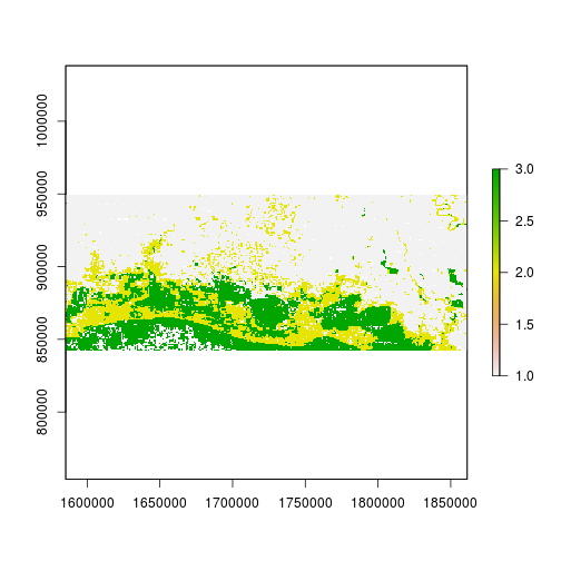
Now predict the subset data based on the model.
raster_out_filename_rp <- file.path(out_dir, paste0("r_predicted_rpart_", out_suffix, file_format))

r_predicted_rpart <- predict(r_stack, mod_rpart, type='class', filename = raster_out_filename_rp,
                             progress = 'text', overwrite = T)
> plot(r_predicted_rpart)
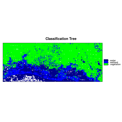
r_predicted_rpart <- ratify(r_predicted_rpart) # creates a raster attribute table (rat)
rat <- levels(r_predicted_rpart)[[1]]
rat$legend <- c("vegetation", "wetland", "water")
levels(r_predicted_rpart) <- rat

levelplot(r_predicted_rpart, maxpixels = 1e6,
          col.regions = c("green","blue","darkblue"),
          scales=list(draw=FALSE),
          main = "Classification Tree")
Support Vector Machine classification (SVM)
Set class_ID as factor to generate classification.
mod_svm <- svm(class_ID ~ Red + NIR + Blue + Green + SWIR1 + SWIR2 + SWIR3,
               data=data_training, method="C-classification",
               kernel="linear") # can be radial
> summary(mod_svm)
Call:
svm(formula = class_ID ~ Red + NIR + Blue + Green + SWIR1 + SWIR2 +
    SWIR3, data = data_training, method = "C-classification", kernel = "linear")


Parameters:
   SVM-Type:  C-classification
 SVM-Kernel:  linear
       cost:  1

Number of Support Vectors:  111

 ( 11 55 45 )


Number of Classes:  3

Levels:
 vegetation wetland water
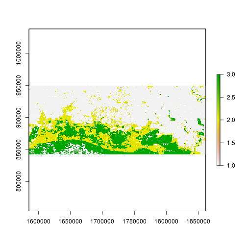
Now predict the subset data based on the model.
raster_out_filename_sv <- file.path(out_dir, paste0("r_predicted_svm_", out_suffix, file_format))

r_predicted_svm <- predict(r_stack, mod_svm, progress = 'text',
                           filename = raster_out_filename_sv, overwrite = T)
plot(r_predicted_svm)
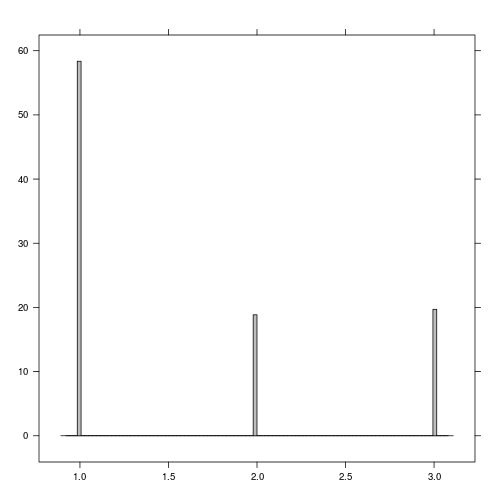
rasterVis::histogram(r_predicted_svm)
r_predicted_svm <- ratify(r_predicted_svm)
rat <- levels(r_predicted_svm)[[1]]
rat$legend <- c("vegetation", "wetland", "water")
levels(r_predicted_svm) <- rat

levelplot(r_predicted_svm, maxpixels = 1e6,
          col.regions = c("green","blue","darkblue"),
          scales = list(draw = FALSE),
          main = "SVM classification")
Part IV: Assessment and comparison of model performance
Set up testing data: Full dataset, let’s use data points for testing.
> dim(data_df)
[1] 1547 16
# omit values that contain NA, because may be problematic with SVM.
data_testing <- na.omit(subset(data_df, training==0))
> dim(data_testing)
[1] 452 16
Predict on testing data using rpart model fitted with testing data.
testing_rpart <- predict(mod_rpart, data_testing, type='class')
Predict on testing data using SVM model fitted with testing data.
testing_svm <- predict(mod_svm, data_testing, type='class')
Predicted number of pixels in each class:
table(testing_rpart)
testing_rpart
vegetation    wetland      water
       153         77        222
table(testing_svm)
testing_svm
vegetation    wetland      water
       152         84        216
Generate confusion matrix to assess the accuracy of the image classification
More info on confusion matrices here: http://spatial-analyst.net/ILWIS/htm/ilwismen/confusion_matrix.htm
Groundtruth data:
> table(data_testing$class_ID)
vegetation    wetland      water
       151         84        217
Classification model results:
> table(testing_rpart)
testing_rpart
vegetation    wetland      water
       153         77        222
> table(testing_svm)
testing_svm
vegetation    wetland      water
       152         84        216
To generate confusion matrix, need to use: testing_rpart: contains classification model prediction in the rows data_testing$class_ID: this column contains groundtruth data
tb_rpart <- table(testing_rpart, data_testing$class_ID)
tb_svm <- table(testing_svm, data_testing$class_ID)
Matrices identifying correct and incorrect classifications by models:
> tb_rpart
testing_rpart vegetation wetland water
   vegetation        148       5     0
   wetland             3      70     4
   water               0       9   213
> tb_svm
testing_svm  vegetation wetland water
  vegetation        151       1     0
  wetland             0      77     7
  water               0       6   210
Accuracy (producer’s accuracy): the fraction of correctly classified pixels compared to all pixels of that groundtruth class.
tb_rpart[1]/sum(tb_rpart[,1]) # producer accuracy
[1] 0.9801325
tb_svm[1]/sum(tb_svm[,1]) # producer accuracy
[1] 1
Looking at accuracy more closely:
# overall accuracy for rpart
sum(diag(tb_rpart))/sum(table(testing_rpart))
[1] 0.9535398
# overall accuracy for svm
sum(diag(tb_svm))/sum(table(testing_svm))
[1] 0.9690265
Generate more accurate measurements from functions in the caret package:
accuracy_info_rpart <- confusionMatrix(testing_rpart, data_testing$class_ID, positive = NULL)
accuracy_info_svm <- confusionMatrix(testing_svm, data_testing$class_ID, positive = NULL)
Overall accuracy produced:
> accuracy_info_rpart$overall
      Accuracy          Kappa  AccuracyLower  AccuracyUpper   AccuracyNull
  9.535398e-01   9.249994e-01   9.298553e-01   9.710138e-01   4.800885e-01
AccuracyPValue  McnemarPValue
 3.536418e-108            NaN
> accuracy_info_svm$overall
      Accuracy          Kappa  AccuracyLower  AccuracyUpper   AccuracyNull
  9.690265e-01   9.503390e-01   9.485775e-01   9.829652e-01   4.800885e-01
AccuracyPValue  McnemarPValue
 3.961900e-118            NaN
Write out the results:
table_out_filename <- file.path(out_dir, "confusion_matrix_rpart.txt")
write.table(accuracy_info_rpart$table, table_out_filename, sep=",")

table_out_filename <- file.path(out_dir, "confusion_matrix_svm.txt")
write.table(accuracy_info_svm$table, table_out_filename, sep=",")
If you need to catch-up before a section of code will work, just squish it's 🍅 to copy code above it into your clipboard. Then paste into your interpreter's console, run, and you'll be ready to start in on that section. Code copied by both 🍅 and 📋 will also appear below, where you can edit first, and then copy, paste, and run again.
# Nothing here yet!