Remote Sensing & Classification
Hurricane Inundation
Lesson 3 with Benoit Parmentier
Contents
####################################  Introduction to Remote Sensing   #######################################
############################  Analyze and map flooding from RITA hurricane  #######################################
#This script performs analyses for the Exercise 5 of the Short Course using reflectance data derived from MODIS.
#The goal is to map flooding from RITA using various reflectance bands from Remote Sensing platforms.
#Additional data is provided including FEMA flood region.
#
#AUTHORS: Benoit Parmentier
#DATE CREATED: 03/05/2018
#DATE MODIFIED: 03/31/2018
#Version: 1
#PROJECT: SESYNC and AAG 2018 Geospatial Short Course and workshop preparation
#TO DO:
#
#COMMIT: clean up of code
#
#################################################################################################

###Loading R library and packages

library(sp) # spatial/geographfic objects and functions
library(rgdal) #GDAL/OGR binding for R with functionalities
rgdal: version: 1.2-18, (SVN revision 718)
 Geospatial Data Abstraction Library extensions to R successfully loaded
 Loaded GDAL runtime: GDAL 2.1.3, released 2017/20/01
 Path to GDAL shared files: /usr/share/gdal/2.1
 GDAL binary built with GEOS: TRUE
 Loaded PROJ.4 runtime: Rel. 4.9.2, 08 September 2015, [PJ_VERSION: 492]
 Path to PROJ.4 shared files: (autodetected)
 Linking to sp version: 1.2-7
library(spdep) #spatial analyses operations, functions etc.
Loading required package: Matrix
Loading required package: spData
To access larger datasets in this package, install the spDataLarge
package with: `install.packages('spDataLarge',
repos='https://nowosad.github.io/drat/', type='source'))`
library(gtools) # contains mixsort and other useful functions
library(maptools) # tools to manipulate spatial data
Checking rgeos availability: TRUE
library(parallel) # parallel computation, part of base package no
library(rasterVis) # raster visualization operations
Loading required package: raster
Loading required package: lattice
Loading required package: latticeExtra
Loading required package: RColorBrewer
library(raster) # raster functionalities
library(forecast) #ARIMA forecasting
library(xts) #extension for time series object and analyses
Loading required package: zoo
Attaching package: 'zoo'
The following objects are masked from 'package:base':

    as.Date, as.Date.numeric
library(zoo) # time series object and analysis
library(lubridate) # dates functionality
Attaching package: 'lubridate'
The following object is masked from 'package:base':

    date
library(colorRamps) #contains matlab.like color palette
library(rgeos) #contains topological operations
rgeos version: 0.3-26, (SVN revision 560)
 GEOS runtime version: 3.5.1-CAPI-1.9.1 r4246
 Linking to sp version: 1.2-5
 Polygon checking: TRUE
library(sphet) #contains spreg, spatial regression modeling
Attaching package: 'sphet'
The following object is masked from 'package:raster':

    distance
library(BMS) #contains hex2bin and bin2hex, Bayesian methods
library(bitops) # function for bitwise operations
library(foreign) # import datasets from SAS, spss, stata and other sources
library(gdata) #read xls, dbf etc., not recently updated but useful
gdata: read.xls support for 'XLS' (Excel 97-2004) files ENABLED.
gdata: read.xls support for 'XLSX' (Excel 2007+) files ENABLED.
Attaching package: 'gdata'
The following objects are masked from 'package:xts':

    first, last
The following objects are masked from 'package:raster':

    resample, trim
The following object is masked from 'package:stats':

    nobs
The following object is masked from 'package:utils':

    object.size
The following object is masked from 'package:base':

    startsWith
library(classInt) #methods to generate class limits
library(plyr) #data wrangling: various operations for splitting, combining data
Attaching package: 'plyr'
The following object is masked from 'package:lubridate':

    here
#library(gstat) #spatial interpolation and kriging methods
library(readxl) #functionalities to read in excel type data
library(psych) #pca/eigenvector decomposition functionalities
Attaching package: 'psych'
The following object is masked from 'package:gtools':

    logit
library(sf) # spatial objects classes
Linking to GEOS 3.5.1, GDAL 2.1.3, proj.4 4.9.2
library(plotrix) #various graphic functions e.g. draw.circle
Attaching package: 'plotrix'
The following object is masked from 'package:psych':

    rescale
###### Functions used in this script
create_dir_fun <- function(outDir,out_suffix=NULL){
#if out_suffix is not null then append out_suffix string
if(!is.null(out_suffix)){
out_name <- paste("output_",out_suffix,sep="")
outDir <- file.path(outDir,out_name)
}
#create if does not exists
if(!file.exists(outDir)){
dir.create(outDir)
}
return(outDir)
}
##### Parameters and argument set up ###########
#in_dir_reflectance <- "data/reflectance_RITA"
in_dir_var <- "../data"
out_dir <- "."
#region coordinate reference system
#http://spatialreference.org/ref/epsg/nad83-texas-state-mapping-system/proj4/
CRS_reg <- "+proj=lcc +lat_1=27.41666666666667 +lat_2=34.91666666666666 +lat_0=31.16666666666667 +lon_0=-100 +x_0=1000000 +y_0=1000000 +ellps=GRS80 +datum=NAD83 +units=m +no_defs"
file_format <- ".tif" # Output format for raster images that are written out.
NA_flag_val <- -9999
out_suffix <-"exercise5_03312018" #output suffix for the files and ouptu folder #PARAM 8
create_out_dir_param <- TRUE
### Input data files used:
infile_reg_outline <- "new_strata_rita_10282017" # Region outline and FEMA zones
infile_modis_bands_information <- "df_modis_band_info.txt" # MOD09 bands information.
nlcd_2006_filename <- "nlcd_2006_RITA.tif" # NLCD2006 Land cover data aggregated at ~ 1km.
infile_name_nlcd_legend <- "nlcd_legend.txt" #Legend information for 2006 NLCD.
#MOD09 surface reflectance product on 2005-09-22 or day of year 2005265
infile_reflectance_date1 <- "mosaiced_MOD09A1_A2005265__006_reflectance_masked_RITA_reg_1km.tif"
#MOD09 surface reflectance product on 2005-09-30 or day of year 2005273
infile_reflectance_date2 <- "mosaiced_MOD09A1_A2005273__006_reflectance_masked_RITA_reg_1km.tif"
################# START SCRIPT ###############################
### PART I: READ AND PREPARE DATA FOR ANALYSES #######
## First create an output directory
if(is.null(out_dir)){
out_dir <- dirname(in_dir) #output will be created in the input dir
}
out_suffix_s <- out_suffix #can modify name of output suffix
if(create_out_dir_param==TRUE){
out_dir <- create_dir_fun(out_dir,out_suffix_s)
setwd(out_dir)
}else{
setwd(out_dir) #use previoulsy defined directory
}
##### PART I: DISPLAY AND EXPLORE DATA ##############
###### Read in MOD09 reflectance images before and after Hurrican Rita.
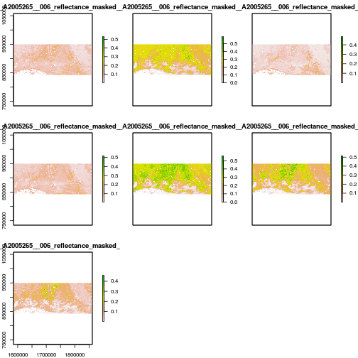
r_before <- brick(file.path(in_dir_var,infile_reflectance_date1)) # Before RITA, Sept. 22, 2005.
r_after <- brick(file.path(in_dir_var,infile_reflectance_date2)) # After RITA, Sept 30, 2005.
plot(r_before) # Note that this is a multibands image.
reg_sf <- st_read(file.path(in_dir_var,infile_reg_outline))
Reading layer `new_strata_rita_10282017' from data source `/nfs/public-data/training/new_strata_rita_10282017' using driver `ESRI Shapefile'
Simple feature collection with 2 features and 17 fields
geometry type:  MULTIPOLYGON
dimension:      XY
bbox:           xmin: -93.92921 ymin: 29.47236 xmax: -91.0826 ymax: 30.49052
epsg (SRID):    4269
proj4string:    +proj=longlat +datum=NAD83 +no_defs
reg_sf <- st_transform(reg_sf,
crs=CRS_reg)
reg_sp <-as(reg_sf, "Spatial") #Convert to sp object before rasterization
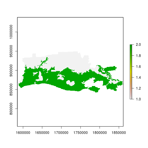
r_ref <- rasterize(reg_sp,
r_before,
field="OBJECTID_1",
fun="first")
plot(r_ref) # zone 2 is flooded and zone 1 is not flooded
#### Let's examine a location within FEMA flooded zone and outside: use centroids
centroids_sf <- st_centroid(reg_sf)
df_before <- extract(r_before,centroids_sf)
df_after <- extract(r_after,centroids_sf)
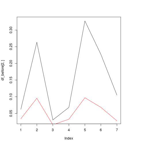
### Plot values of bands before and after for flooded region:
plot(df_before[2,],type="l")
lines(df_after[2,],col="red")
## Read band information since it is more informative!!
df_modis_band_info <- read.table(file.path(in_dir_var,infile_modis_bands_information),
                                 sep=",",
                                 stringsAsFactors = F)
print(df_modis_band_info)
  band_name band_number start_wlength end_wlength
1       Red           3           620         670
2       NIR           4           841         876
3      Blue           1           459         479
4     Green           2           545         565
5     SWIR1           5          1230        1250
6     SWIR2           6          1628        1652
7     SWIR3           7          2105        2155
names(r_before) <- df_modis_band_info$band_name
names(r_after) <- df_modis_band_info$band_name
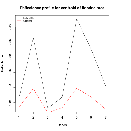
### Order band in terms of wavelenth:
df_modis_band_info <- df_modis_band_info[order(df_modis_band_info$start_wlength),]
#SWIR1 (1230–1250 nm), SWIR2 (1628–1652 nm) and SWIR3 (2105–2155 nm).
band_refl_order <- df_modis_band_info$band_number
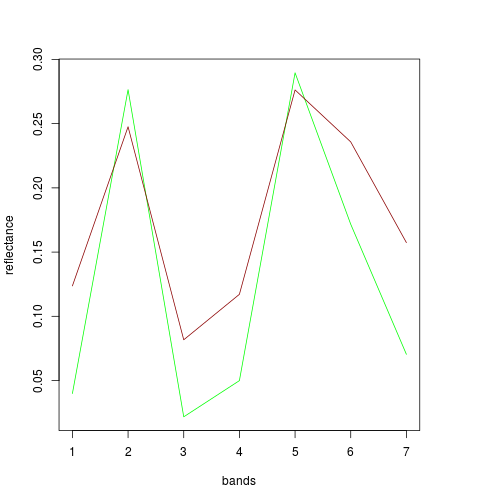
plot(df_before[2,band_refl_order],type="l",
xlab="Bands",
ylab="Reflectance",
main="Reflectance profile for centroid of flooded area")
lines(df_after[2,band_refl_order],col="red")
names_vals <- c("Before Rita","After Rita")
legend("topleft",legend=names_vals,
pt.cex=0.7,cex=0.7,col=c("black","red"),
lty=1, #add circle symbol to line
bty="n")
###############################################
##### PART II: Examine spectral class signatures for land cover NLCD classes ##############

###### Read in NLDC 2006, note that it was aggregated at 1km.
nlcd2006_reg <- raster(file.path(in_dir_var,nlcd_2006_filename))
#### Extract zonal averages by NLCD classes using zonal raster
avg_reflectance_nlcd <- as.data.frame(zonal(r_before,nlcd2006_reg,fun="mean"))

#### read in NLCD legend to add to the average information
lc_legend_df <- read.table(file.path(in_dir_var,infile_name_nlcd_legend),
                           stringsAsFactors = F,
                           sep=",")
print(avg_reflectance_nlcd)
   zone        Red        NIR       Blue      Green      SWIR1      SWIR2
1     0 0.03458904 0.01535499 0.03581749 0.05163573 0.01262342 0.01771813
2    11 0.07307984 0.06784635 0.06036733 0.07956521 0.05991636 0.04664948
3    21 0.07276522 0.28171285 0.04420428 0.07726309 0.31805232 0.23408753
4    22 0.08235028 0.27960481 0.05117458 0.08538413 0.30907538 0.23123385
5    23 0.10574247 0.26636831 0.06789142 0.10388469 0.29315783 0.23319375
6    24 0.12368051 0.24758425 0.08174059 0.11712968 0.27622949 0.23576209
7    31 0.09874217 0.13020133 0.07870421 0.09989436 0.12222435 0.09422932
8    41 0.05644301 0.26516752 0.03530746 0.06259356 0.28388245 0.18083792
9    42 0.03990187 0.27645189 0.02177976 0.04993706 0.28957741 0.17166508
10   43 0.03941129 0.28346313 0.02211763 0.05035833 0.30668417 0.18516430
11   52 0.04540521 0.27760067 0.02405570 0.05334825 0.30194988 0.19117841
12   71 0.05569214 0.27195001 0.03005173 0.06076262 0.30610093 0.20940236
13   81 0.07483913 0.27795804 0.04250243 0.07692526 0.32523050 0.24754272
14   82 0.08456354 0.27472078 0.04777970 0.08379540 0.31051877 0.24309384
15   90 0.03852322 0.23273819 0.02317667 0.04775357 0.25516940 0.15667656
16   95 0.06208044 0.19687418 0.03674701 0.06434722 0.21390883 0.15373826
        SWIR3
1  0.01260556
2  0.02672107
3  0.11926512
4  0.12615517
5  0.14802151
6  0.15738439
7  0.05498403
8  0.07959769
9  0.07041540
10 0.07498740
11 0.08314305
12 0.09997039
13 0.12366634
14 0.13108070
15 0.06237482
16 0.07421595
names(lc_legend_df)
[1] "ID"                         "COUNT"
[3] "Red"                        "Green"
[5] "Blue"                       "NLCD.2006.Land.Cover.Class"
[7] "Opacity"
### Add relevant categories
lc_legend_df_subset <- subset(lc_legend_df,select=c("ID","NLCD.2006.Land.Cover.Class"))
names(lc_legend_df_subset) <- c("ID","cat_name")

avg_reflectance_nlcd <- merge(avg_reflectance_nlcd,lc_legend_df_subset,by.x="zone",by.y="ID",all.y=F)
head(avg_reflectance_nlcd)
  zone        Red        NIR       Blue      Green      SWIR1      SWIR2
1    0 0.03458904 0.01535499 0.03581749 0.05163573 0.01262342 0.01771813
2   11 0.07307984 0.06784635 0.06036733 0.07956521 0.05991636 0.04664948
3   21 0.07276522 0.28171285 0.04420428 0.07726309 0.31805232 0.23408753
4   22 0.08235028 0.27960481 0.05117458 0.08538413 0.30907538 0.23123385
5   23 0.10574247 0.26636831 0.06789142 0.10388469 0.29315783 0.23319375
6   24 0.12368051 0.24758425 0.08174059 0.11712968 0.27622949 0.23576209
       SWIR3                    cat_name
1 0.01260556                Unclassified
2 0.02672107                  Open Water
3 0.11926512       Developed, Open Space
4 0.12615517    Developed, Low Intensity
5 0.14802151 Developed, Medium Intensity
6 0.15738439   Developed, High Intensity
names(avg_reflectance_nlcd)
[1] "zone"     "Red"      "NIR"      "Blue"     "Green"    "SWIR1"
[7] "SWIR2"    "SWIR3"    "cat_name"
col_ordering <- band_refl_order + 1

plot(as.numeric(avg_reflectance_nlcd[9,col_ordering]),
     type="l",
     col="green",
     xlab="bands",
     ylab="reflectance") #42 evergreen forest
lines(as.numeric(avg_reflectance_nlcd[6,col_ordering]),
      type="l",
      col="darkred") #22 developed,High intensity
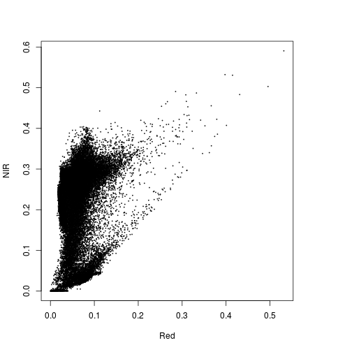
####### Explore data in Feature space:

#Feature space NIR1 and Red
plot(r_before$Red, r_before$NIR)
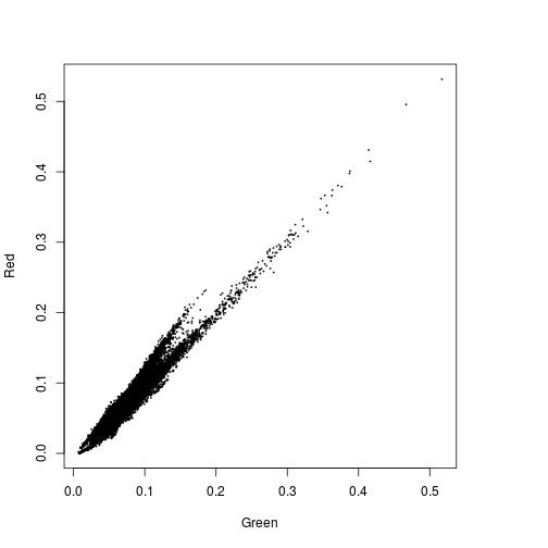
plot(r_before$Green,r_before$Red)
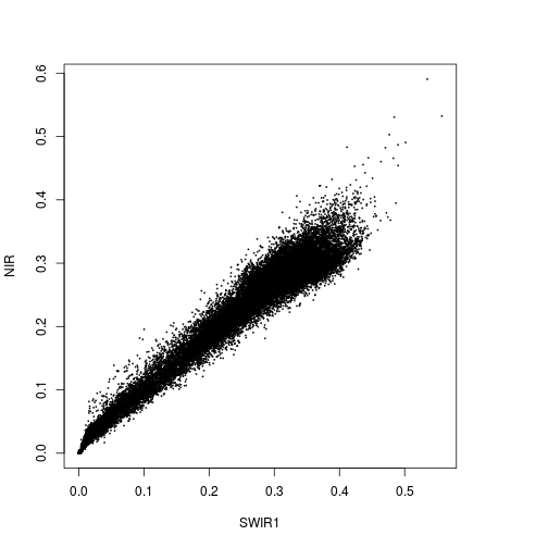
plot(r_before$SWIR1,r_before$NIR)
plot(r_before$Red,r_before$SWIR1)
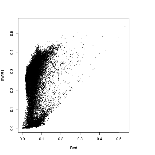
df_r_before_nlcd <- as.data.frame(stack(r_before,nlcd2006_reg))
head(df_r_before_nlcd)
         Red       NIR       Blue      Green     SWIR1     SWIR2
1 0.03599200 0.2599244 0.02133671 0.04703750 0.2810231 0.1553841
2 0.02928869 0.2715889 0.01696460 0.04409311 0.2720489 0.1396950
3 0.02671438 0.2838178 0.01695321 0.04189149 0.2874987 0.1507025
4 0.02691096 0.2825994 0.01606729 0.04149844 0.2870458 0.1528974
5 0.04274514 0.2800327 0.02311076 0.05212086 0.3009017 0.1827510
6 0.03583299 0.2768207 0.02156925 0.04826682 0.2877768 0.1600456
       SWIR3 nlcd_2006_RITA
1 0.05624928             NA
2 0.04715122             NA
3 0.04982105             NA
4 0.05246148             NA
5 0.07394192             NA
6 0.05998935             NA
#Evergreen Forest:
df_subset <- subset(df_r_before_nlcd,nlcd_2006_RITA==42)
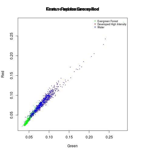
plot(df_subset$Green,
df_subset$Red,
col="green",
cex=0.15,
xlab="Green",
ylab="Red",
main="Green-Red feature space")
#Urban: dense
df_subset <- subset(df_r_before_nlcd,nlcd_2006_RITA==22)
points(df_subset$Green,
df_subset$Red,
col="darkred",
cex=0.15)
#Water: 11 for NLCD
df_subset <- subset(df_r_before_nlcd,nlcd_2006_RITA==22)
points(df_subset$Green,
df_subset$Red,
col="blue",
cex=0.15)
title("Feature space Green-Red")
names_vals <- c("Evergreen Forest","Developed High Intensity","Water")
legend("topright",legend=names_vals,
pt.cex=0.7,cex=0.7,col=c("green","darkred","blue"),
pch=1, #add circle symbol to line
bty="n")
#### Feature space Red and NIR
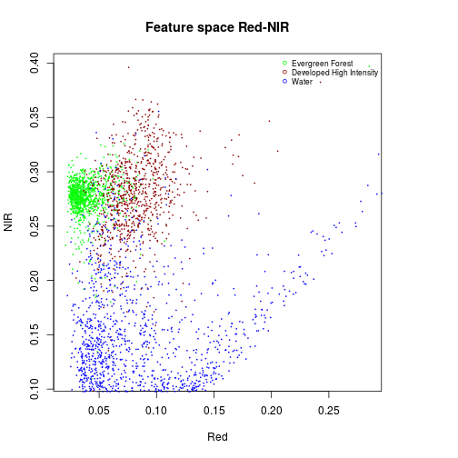
#Evergreen Forest:
df_subset <- subset(df_r_before_nlcd,nlcd_2006_RITA==42)
plot(df_subset$Red,
df_subset$NIR,
col="green",
cex=0.15,
xlab="Red",
ylab="NIR")
#Developed, High Intensity
df_subset <- subset(df_r_before_nlcd,nlcd_2006_RITA==22)
points(df_subset$Red,
df_subset$NIR,
col="darkred",
cex=0.15)
#Water
df_subset <- subset(df_r_before_nlcd,nlcd_2006_RITA==11)
points(df_subset$Red,
df_subset$NIR,
col="blue",
cex=0.15)
title("Feature space Red-NIR")
names_vals <- c("Evergreen Forest","Developed High Intensity","Water")
legend("topright",legend=names_vals,
pt.cex=0.7,cex=0.7,col=c("green","darkred","blue"),
pch=1, #add circle symbol to line
bty="n")
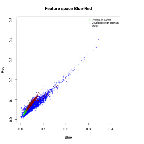
#### Feature space Blue and Red

#Water:
df_subset <- subset(df_r_before_nlcd,nlcd_2006_RITA==11)
plot(df_subset$Blue,
       df_subset$Red,
       col="blue",
       cex=0.15,
       xlab="Blue",
       ylab="Red")

#Evergreen Forest:
df_subset <- subset(df_r_before_nlcd,nlcd_2006_RITA==42)
points(df_subset$Blue,
       df_subset$Red,
       col="green",
       cex=0.15)

#Urban dense:
df_subset <- subset(df_r_before_nlcd,nlcd_2006_RITA==22)
points(df_subset$Blue,
       df_subset$Red,
       col="darkred",
       cex=0.15)

title("Feature space Blue-Red")
names_vals <- c("Evergreen Forest","Developed High Intensity","Water")
legend("topright",legend=names_vals,
       pt.cex=0.7,cex=0.7,col=c("green","darkred","blue"),
       pch=1, #add circle symbol to line
       bty="n")
#### Generate Color composites
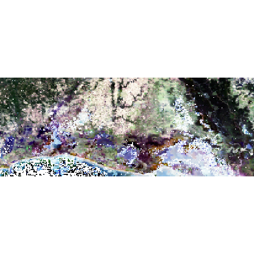
### True color composite
plotRGB(r_before,
r=1,
g=4,
b=3,
scale=0.6,
stretch="hist")
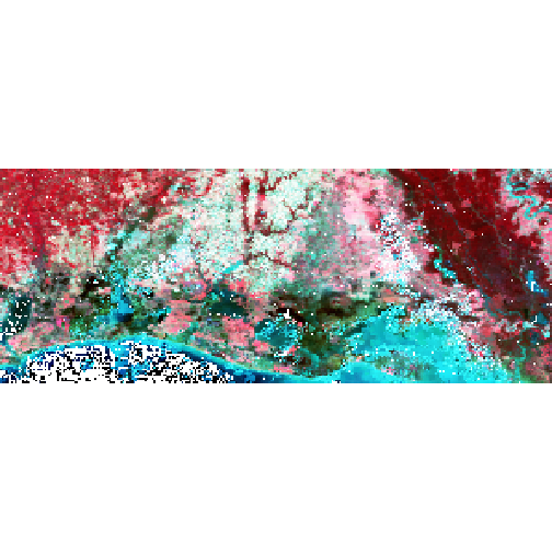
### False color composite:

plotRGB(r_before,
        r=2,
        g=1,
        b=4,
        scale=0.6,
        stretch="hist")
plotRGB(r_after,
        r=2,
        g=1,
        b=4,
        scale=0.6,
        stretch="hist")
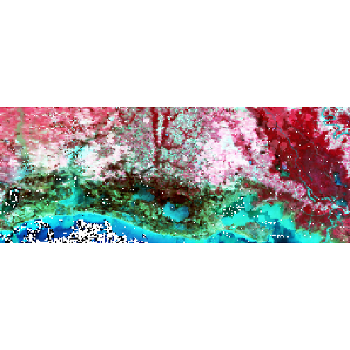
### Note the effect of flooding is particularly visible in the false color composites.
### Let's examine different band combination to enhance features in the image, including flooded areas.

###############################################
##### PART III: Band combination: Indices and thresholding for flood mapping ##############

### NIR experiment with threshold to  map water/flooding

plot(subset(r_before,"NIR"))
plot(subset(r_after,"NIR"))
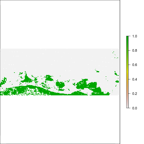
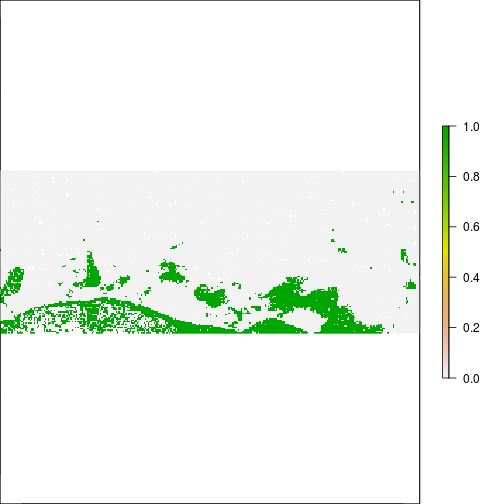
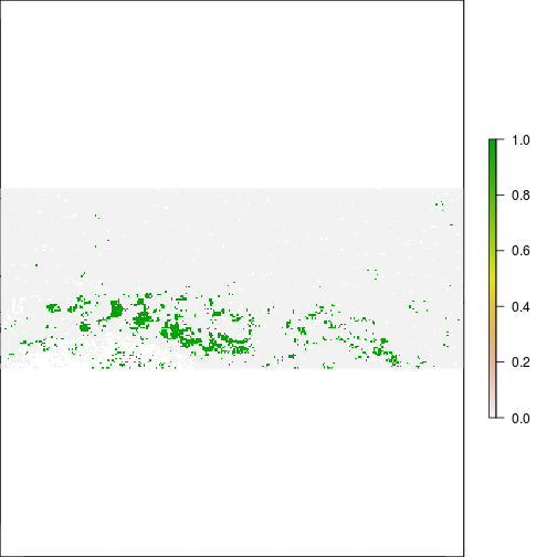
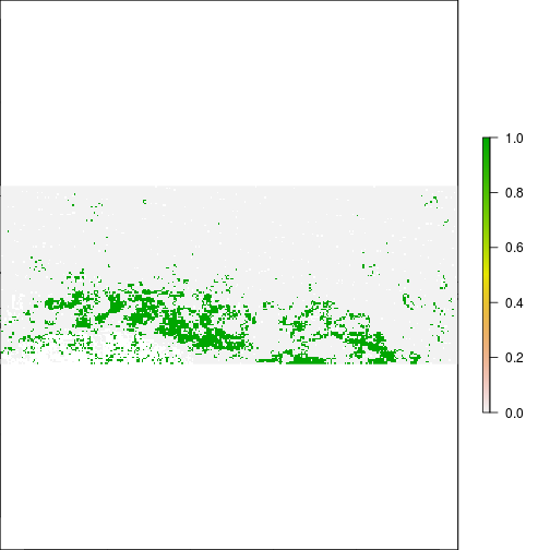
### Lower NIR often correlates to areas with high water fraction or inundated:
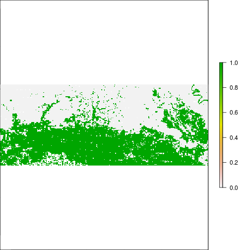
r_rec_NIR_before <- subset(r_before,"NIR") < 0.2
r_rec_NIR_after <- subset(r_after,"NIR") < 0.2
### THis is suggesting flooding!!!
plot(r_rec_NIR_before, main="Before RITA, NIR > 0.2")
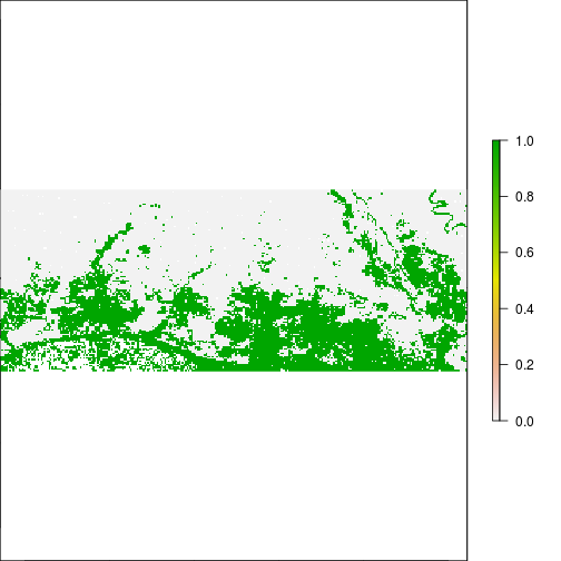
plot(r_rec_NIR_after, main="After RITA, NIR > 0.2")
#Compare to actual flooding data
freq_fema_zones <- as.data.frame(freq(r_ref))
xtab_threshold <- crosstab(r_ref,r_rec_NIR_after,long=T)

## % overlap between the flooded area and values below 0.2 in NIR
(xtab_threshold[5,3]/freq_fema_zones[2,2])*100 #agreement with FEMA flooded area in %.
[1] 76.17498
############## Generating indices based on raster algebra of original bands
## Let's generate a series of indices, we list a few possibility from the literature.
#1) NDVI = (NIR - Red)/(NIR+Red)
#2) NDWI = (Green - NIR)/(Green + NIR)
#3) MNDWI = Green - SWIR2 / Green + SWIR2
#4) NDWI2 (LSWIB5) =  (NIR - SWIR1)/(NIR + SWIR1)
#5) LSWI (LSWIB5) =  (NIR - SWIR2)/(NIR + SWIR2)

names(r_before)
[1] "Red" "NIR" "Blue" "Green" "SWIR1" "SWIR2" "SWIR3"
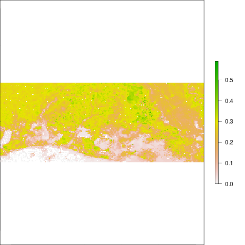
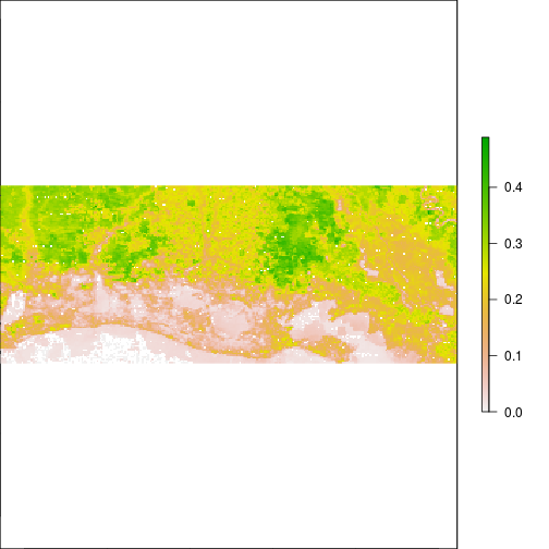
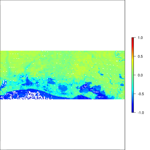
r_before_NDVI <- (r_before$NIR - r_before$Red) / (r_before$NIR + r_before$Red)
r_after_NDVI <- subset(r_after,"NIR") - subset(r_after,"Red")/(subset(r_after,"NIR") + subset(r_after,"Red"))

plot(r_before_NDVI,zlim=c(-1,1),col=matlab.like(255))
plot(r_after_NDVI,zlim=c(-1,1),col=matlab.like2(255))
### Experiment with different threshold values:
# THis is suggesting flooding!!!
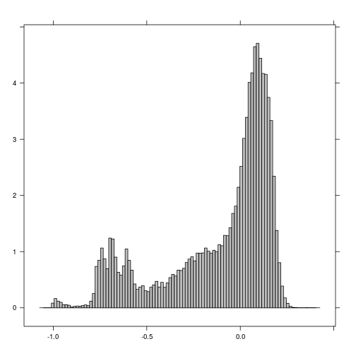
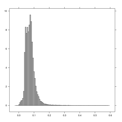
histogram(r_before_NDVI) # Examine histogram to look for potential threshold values
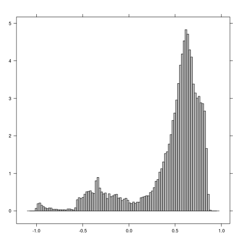
histogram(r_after_NDVI) # Examine histogram to look for poential threshold values
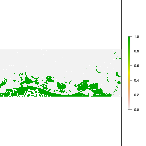
plot(r_before_NDVI < -0.5)
plot(r_after_NDVI < -0.5)
plot(r_before_NDVI < -0.1)
plot(r_after_NDVI < -0.1)
#2) NDWI = (Green - NIR)/(Green + NIR)
#3) MNDWI = Green - SWIR2 / Green + SWIR2
#Modified NDWI known as MNDWI : Green - SWIR2/(Green + SWIR2)
#According to Gao (1996), NDWI is a good indicator for vegetation liquid water content and
# is less sensitive to atmospheric scattering effects than NDVI. In some studies, MODIS band 6
# is used for the NDWI calculation, because it is sensitive to water types and contents
# (Li et al., 2011), while band 5 is sensitive to vegetation liquid water content (Gao, 1996).
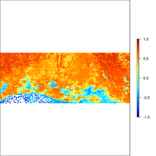
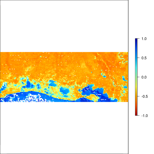
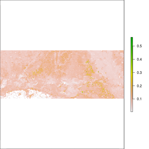
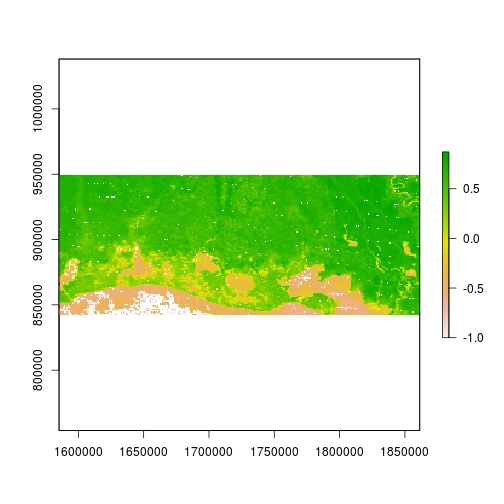
r_before_MNDWI <- (r_before$Green - r_before$SWIR2) / (r_before$Green + r_before$SWIR2)
r_after_MNDWI <- (r_after$Green - r_after$SWIR2) / (r_after$Green + r_after$SWIR2)
plot(r_before_MNDWI,zlim=c(-1,1),col=rev(matlab.like(255)))
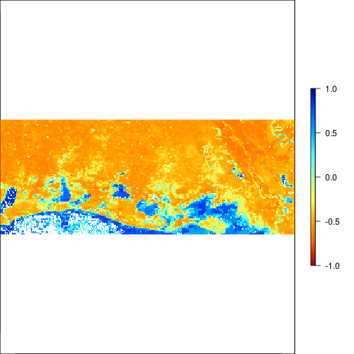
plot(r_after_MNDWI,zlim=c(-1,1),col=rev(matlab.like(255)))
### THis is suggesting flooding!!!
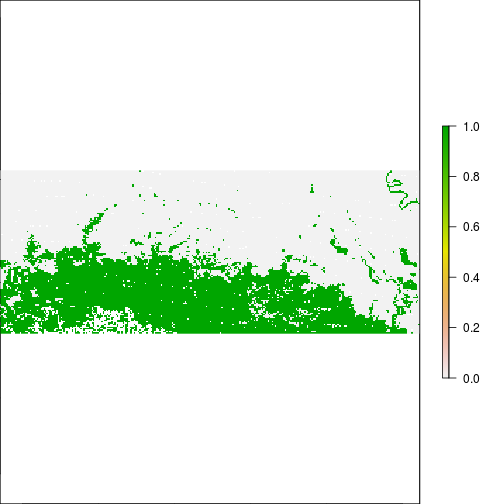
plot(r_before_MNDWI > 0.5)
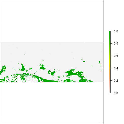
plot(r_after_MNDWI > 0.5)
plot(r_before_MNDWI > 0.1)
plot(r_after_MNDWI > 0.1)
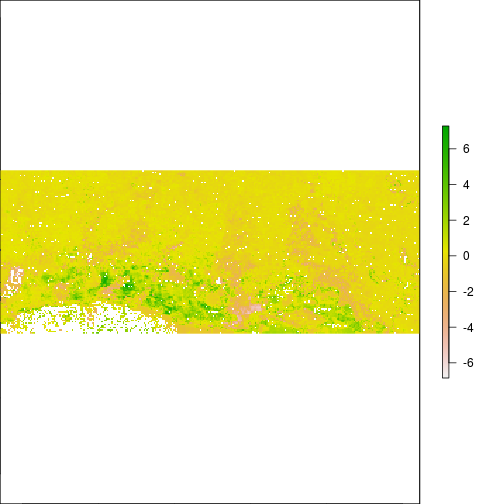
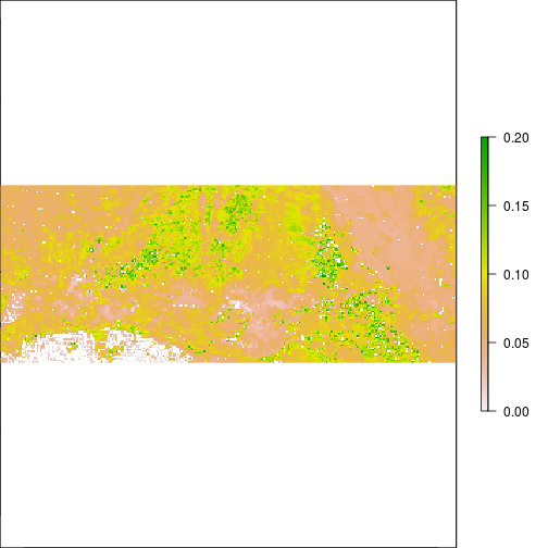
r_diff_MNDWI <- r_after_MNDWI - r_before_MNDWI
plot(r_diff_MNDWI)
plot(r_diff_MNDWI > 0.2) ## Increase in MNDWI: Areas that may have become flooded

#Standardize image:
mean_val <- cellStats(r_diff_MNDWI,"mean")
sd_val <- cellStats(r_diff_MNDWI,"sd")
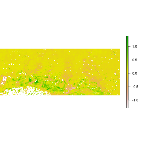
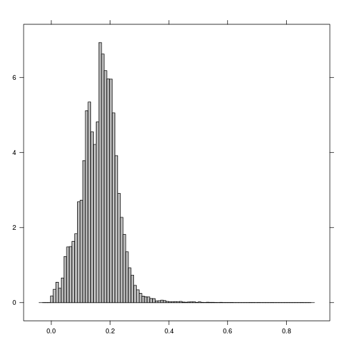
r_diff_std <- (r_diff_MNDWI - mean_val)/ sd_val
plot(r_diff_std)
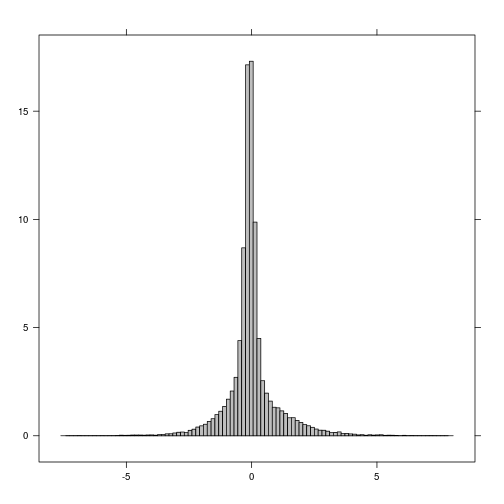
histogram(r_diff_std)
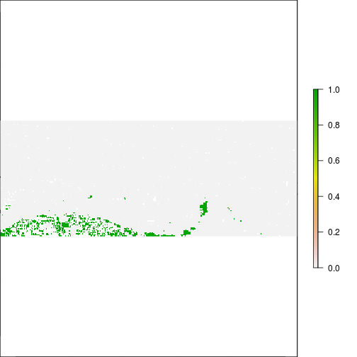
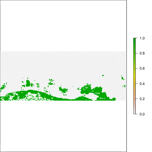
plot(r_diff_std > 2) ## increase in MNDWI 2 standard deiation away
plot(r_diff_std > 1) ## increase in MNDWI 2 standard deiation away
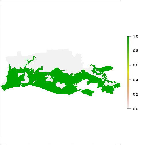
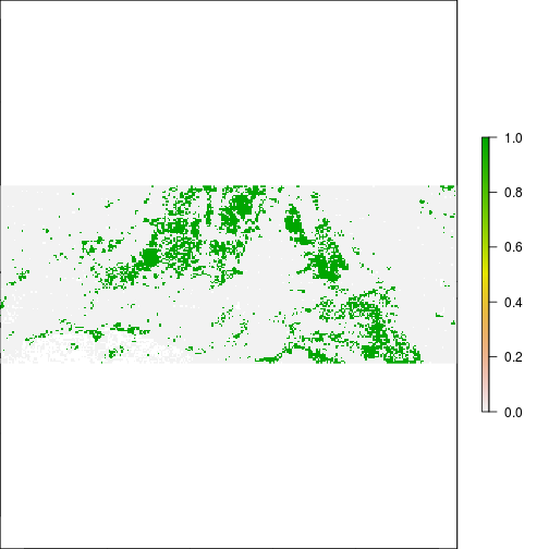
### Generate a map of flooding with MNDWI and compare to FEMA map:

r_after_flood <- r_diff_std > 1
plot(r_after_flood)

#reclass in zero/1!!!

df <- data.frame(id=c(1,2), v=c(0,1))
r_ref_rec <- subs(r_ref, df)
plot(r_ref_rec)
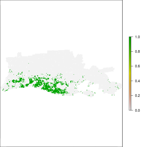
xtab_tb <- crosstab(r_after_flood,r_ref_rec)

## Examine overlap between flooded area and FEMA:

plot(r_after_flood)

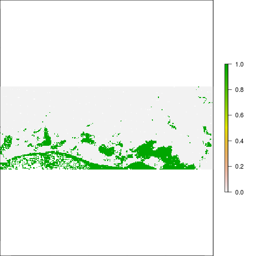
r_overlap <- r_ref_rec * r_after_flood
plot(r_overlap) ## Flood map area of aggreement with FEMA
###############################################
##### PART IV: Principal Component Analysis and band transformation
## Another avenue to combine original bands into indices is to use linear transformation.
## We examine Principal Component Analysis and the Tassel Cap Transform.

#Correlate long term mean to PC!
cor_mat_layerstats <- layerStats(r_before, 'pearson', na.rm=T)
cor_matrix <- cor_mat_layerstats$`pearson correlation coefficient`
class(cor_matrix)
[1] "matrix"
print(cor_matrix) #note size is 7x7
            Red       NIR         Blue     Green        SWIR1     SWIR2
Red   1.0000000 0.2398870  0.903113075 0.9707865  0.256771113 0.4605483
NIR   0.2398870 1.0000000  0.013412596 0.2318272  0.978567657 0.8911699
Blue  0.9031131 0.0134126  1.000000000 0.9498225 -0.002725252 0.1571903
Green 0.9707865 0.2318272  0.949822516 1.0000000  0.218488306 0.3842003
SWIR1 0.2567711 0.9785677 -0.002725252 0.2184883  1.000000000 0.9474207
SWIR2 0.4605483 0.8911699  0.157190340 0.3842003  0.947420706 1.0000000
SWIR3 0.6443259 0.7292226  0.343071136 0.5438923  0.805069686 0.9448527
          SWIR3
Red   0.6443259
NIR   0.7292226
Blue  0.3430711
Green 0.5438923
SWIR1 0.8050697
SWIR2 0.9448527
SWIR3 1.0000000
pca_mod <- principal(cor_matrix,nfactors=7,rotate="none")
class(pca_mod$loadings)
[1] "loadings"
print(pca_mod$loadings)
Loadings:
      PC1    PC2    PC3    PC4    PC5    PC6    PC7
Red    0.774  0.616
NIR    0.779 -0.556  0.282
Blue   0.551  0.812  0.140  0.131
Green  0.734  0.665  0.101
SWIR1  0.806 -0.576  0.123
SWIR2  0.905 -0.403 -0.121
SWIR3  0.933 -0.162 -0.315

                 PC1   PC2   PC3   PC4   PC5   PC6   PC7
SS loadings    4.387 2.310 0.246 0.034 0.011 0.010 0.003
Proportion Var 0.627 0.330 0.035 0.005 0.002 0.001 0.000
Cumulative Var 0.627 0.957 0.992 0.997 0.998 1.000 1.000
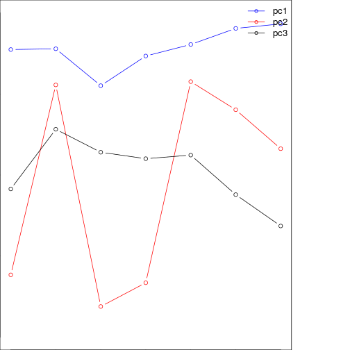
plot(pca_mod$loadings[,1][band_refl_order],type="b",
     xlab="time steps",
     ylab="PC loadings",
     ylim=c(-1,1),
     col="blue")
lines(-1*(pca_mod$loadings[,2][band_refl_order]),type="b",col="red")
lines(pca_mod$loadings[,3][band_refl_order],type="b",col="black")
title("Loadings for the first three components using T-mode")

##Make this a time series
loadings_df <- as.data.frame(pca_mod$loadings[,1:7])
title("Loadings for the first three components using T-mode")
names_vals <- c("pc1","pc2","pc3")
legend("topright",legend=names_vals,
       pt.cex=0.8,cex=1.1,col=c("blue","red","black"),
       lty=c(1,1), # set legend symbol as lines
       pch=1, #add circle symbol to line
       lwd=c(1,1),bty="n")
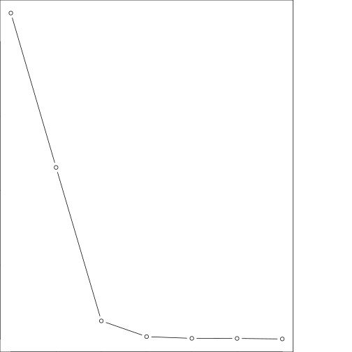
## Add scree plot
plot(pca_mod$values,main="Scree plot: Variance explained",type="b")
### Generate scores from eigenvectors
### Using predict function: this is recommended for raster.
r_pca <- predict(r_before, pca_mod, index=1:7,filename="pc_scores.tif",overwrite=T) # fast
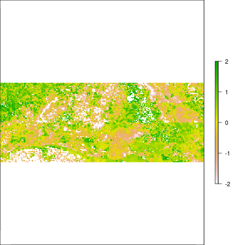
plot(r_pca,y=2,zlim=c(-2,2))
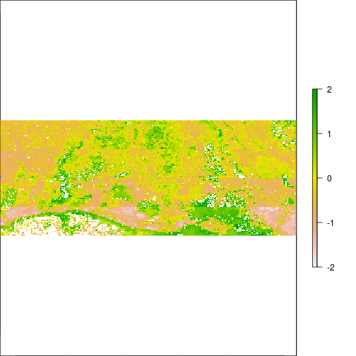
plot(r_pca,y=1,zlim=c(-2,2))
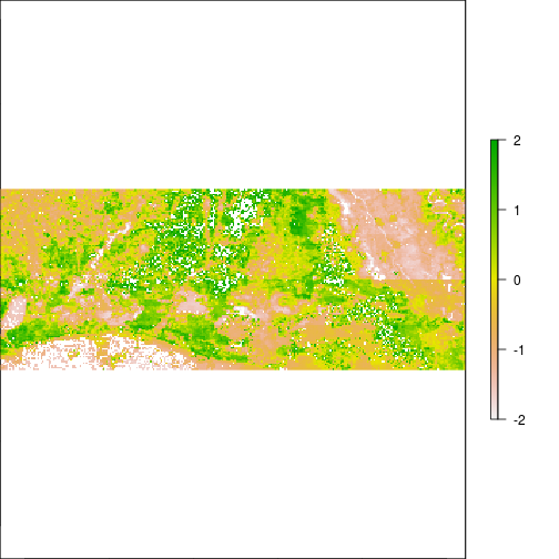
plot(r_pca,y=3,zlim=c(-2,2))
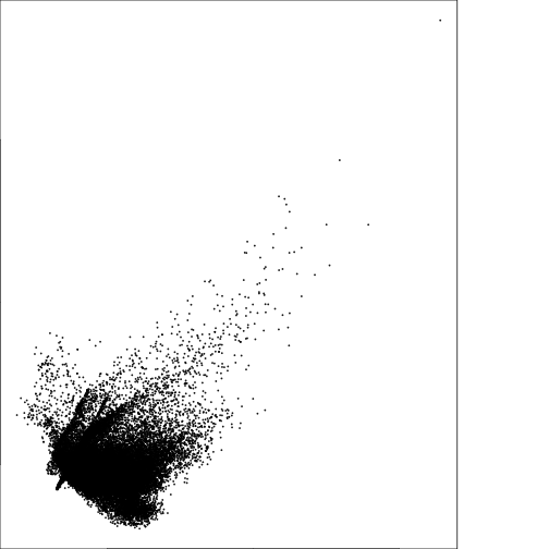
plot(subset(r_pca,1),subset(r_pca,2))
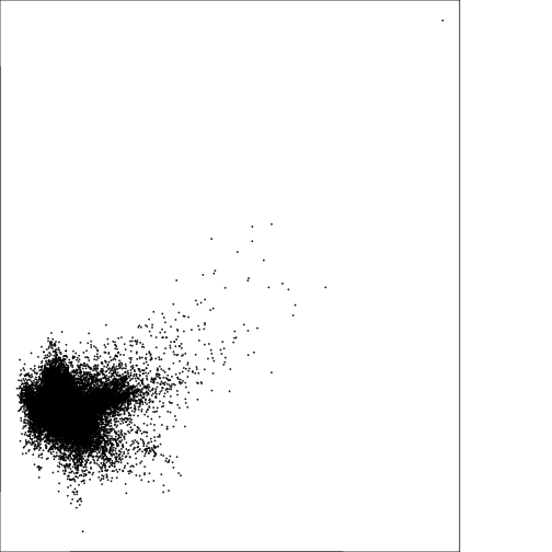
plot(subset(r_pca,2),subset(r_pca,3))
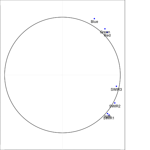
#### Generate a plot for PCA with loadings and compare to Tassel Cap

var_labels <- rownames(loadings_df)

plot(loadings_df[,1],loadings_df[,2],
     type="p",
     pch = 20,
     col ="blue",
     xlab=names(loadings_df)[1],
     ylab=names(loadings_df)[2],
     ylim=c(-1,1),
     xlim=c(-1,1),
     axes = FALSE,
     cex.lab = 1.2)
axis(1, at=seq(-1,1,0.2),cex=1.2)
axis(2, las=1,at=seq(-1,1,0.2),cex=1.2) # "1' for side=below, the axis is drawned  on the right at location 0 and 1

box()    #This draws a box...

title(paste0("Loadings for component ", names(loadings_df)[1]," and " ,names(loadings_df)[2] ))
draw.circle(0,0,c(1.0,1.0),nv=500)#,border="purple",
text(loadings_df[,1],loadings_df[,2],var_labels,pos=1,cex=1)
grid(2,2)
##### plot feature space:

df_raster_val <- as.data.frame(stack(r_after,r_pca,nlcd2006_reg))
head(df_raster_val)
         Red       NIR       Blue      Green     SWIR1     SWIR2
1 0.04558113 0.3027903 0.02379627 0.05476730 0.3318335 0.1902746
2 0.04460510 0.3043112 0.02354558 0.05586702 0.3138186 0.1842244
3 0.04348749 0.2998908 0.02374887 0.05381133 0.3123330 0.1855501
4 0.04507260 0.3017146 0.02426019 0.05503851 0.3193893 0.1913280
5 0.04715690 0.3239896 0.02511090 0.05962222 0.3417773 0.1930779
6 0.03485106 0.2683164 0.01941371 0.04450204 0.2855803 0.1609111
       SWIR3 pc_scores.1 pc_scores.2 pc_scores.3 pc_scores.4 pc_scores.5
1 0.07314926  -0.7644424  -0.1749840   0.4895376  -0.3940996  -0.7156922
2 0.06792310  -0.9065449  -0.3173643   0.9340215  -1.2679656  -3.0844703
3 0.07248760  -0.7900366  -0.5316336   1.2609810  -0.8686562  -2.8946190
4 0.07654412  -0.7877789  -0.5503042   1.1144350  -0.9439425  -2.8750505
5 0.07032830  -0.3890644  -0.3253821   0.6932408  -0.6264383  -1.0684590
6 0.05962812  -0.6346722  -0.3010963   0.9234368  -0.6627523  -2.1239798
  pc_scores.6 pc_scores.7 nlcd_2006_RITA
1   0.9251045  1.48893476             NA
2   1.4692621  0.02715476             NA
3   1.9787420 -0.02099684             NA
4   1.8841606 -0.05822323             NA
5   1.0431399  0.46276042             NA
6   1.4554931  0.37810266             NA
#Water
plot(df_raster_val[df_raster_val$nlcd_2006_RITA==11,c("pc_scores.1")],
     df_raster_val[df_raster_val$nlcd_2006_RITA==11,c("pc_scores.2")],
     col="blue",cex=0.15,
     ylim=c(-2,2),
     xlim=c(-2,2))

#Urban: dense
points(df_raster_val[df_raster_val$nlcd_2006_RITA==22,c("pc_scores.1")],
       df_raster_val[df_raster_val$nlcd_2006_RITA==22,c("pc_scores.2")],
       col="brown",cex=0.15)

#Forest:
points(df_raster_val[df_raster_val$nlcd_2006_RITA==42,c("pc_scores.1")],
       df_raster_val[df_raster_val$nlcd_2006_RITA==42,c("pc_scores.2")],
       col="green",cex=0.15)
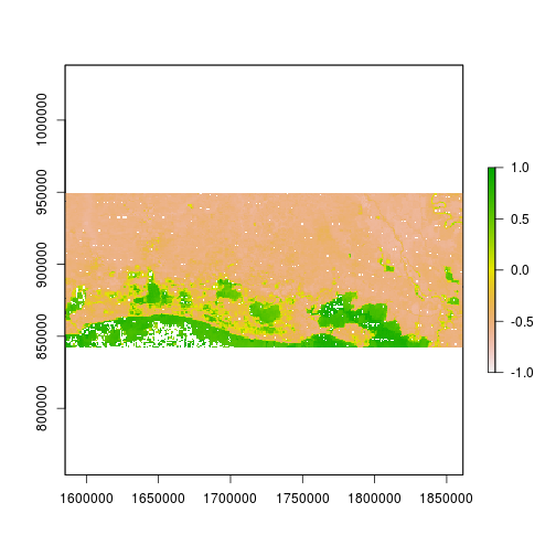
### Note the negative values are related to Forest and positve to water on PC2
plot(r_pca$pc_scores.2 > 0.1) #water related?
plot(r_pca$pc_scores.2 < - 0.1) #vegetation related?
#### Examine relationship with Tasselcap transform adapted for MODIS:
#6) TCWI = 0.10839 * Red+ 0.0912 * NIR +0.5065 * Blue+ 0.404 * Green
# - 0.241 * SWIR1- 0.4658 * SWIR2-
# 0.5306 * SWIR3
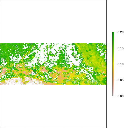
#7) TCBI = 0.3956 * Red + 0.4718 * NIR +0.3354 * Blue+ 0.3834 * Green
# + 0.3946 * SWIR1 + 0.3434 * SWIR2+ 0.2964 * SWIR3
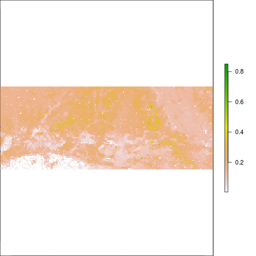
r_TCWI = 0.10839 * r_before$Red + 0.0912 * r_before$NIR +0.5065 * r_before$Blue+ 0.404 * r_before$Green
- 0.241 * r_before$SWIR1- 0.4658 * r_before$SWIR2 - 0.5306 * r_before$SWIR3
class       : RasterLayer
dimensions  : 116, 298, 34568  (nrow, ncol, ncell)
resolution  : 926.6254, 926.6254  (x, y)
extent      : 1585224, 1861359, 842226.7, 949715.2  (xmin, xmax, ymin, ymax)
coord. ref. : +proj=lcc +lat_1=27.41666666666667 +lat_2=34.91666666666666 +lat_0=31.16666666666667 +lon_0=-100 +x_0=1000000 +y_0=1000000 +ellps=GRS80 +towgs84=0,0,0,0,0,0,0 +units=m +no_defs
data source : in memory
names       : layer
values      : -0.5969822, -0.00232494  (min, max)
r_TCBI = 0.3956 * r_before$Red + 0.4718 * r_before$NIR +0.3354 * r_before$Blue+ 0.3834 * r_before$Green
          + 0.3946 * r_before$SWIR1 + 0.3434 * r_before$SWIR2+ 0.2964 * r_before$SWIR3
class       : RasterLayer
dimensions  : 116, 298, 34568  (nrow, ncol, ncell)
resolution  : 926.6254, 926.6254  (x, y)
extent      : 1585224, 1861359, 842226.7, 949715.2  (xmin, xmax, ymin, ymax)
coord. ref. : +proj=lcc +lat_1=27.41666666666667 +lat_2=34.91666666666666 +lat_0=31.16666666666667 +lon_0=-100 +x_0=1000000 +y_0=1000000 +ellps=GRS80 +towgs84=0,0,0,0,0,0,0 +units=m +no_defs
data source : in memory
names       : layer
values      : 0.00172096, 0.4989139  (min, max)
#r_TCWI <- r_TCWI*10
histogram(r_TCWI)
plot(r_TCWI)
plot(r_TCWI,zlim=c(0,0.2))
plot(r_TCWI>0.1)
histogram(r_TCBI)
plot(r_TCBI)
plot(r_TCBI,zlim=c(0,0.2))
r_stack <- stack(r_TCWI,r_TCBI, r_pca)
names(r_stack) <- c("TCWI","TCBI",names(r_pca))
cor_r_TC <- layerStats(r_stack,"pearson",na.rm=T)
cor_r_TC <- as.data.frame(cor_r_TC$`pearson correlation coefficient`)
print(cor_r_TC)
                  TCWI         TCBI pc_scores.1  pc_scores.2 pc_scores.3
TCWI        1.00000000 0.8283253068  0.83971868  0.548005396  0.26578247
TCBI        0.82832531 1.0000000000  0.87114254  0.106891136  0.28142299
pc_scores.1 0.83971868 0.8711425415  1.00000000  0.082280569  0.13336455
pc_scores.2 0.54800540 0.1068911362  0.08228057  1.000000000  0.02282614
pc_scores.3 0.26578247 0.2814229943  0.13336455  0.022826135  1.00000000
pc_scores.4 0.13531034 0.1067056440  0.25180545 -0.008046805 -0.26120385
pc_scores.5 0.06877618 0.0001461868  0.14499957  0.078513273 -0.28695036
pc_scores.6 0.14641088 0.1400215251  0.06428065  0.070531136  0.32528627
pc_scores.7 0.03469429 0.0428780431  0.11454351 -0.114043686  0.03411671
             pc_scores.4   pc_scores.5 pc_scores.6 pc_scores.7
TCWI         0.135310342  0.0687761767  0.14641088  0.03469429
TCBI         0.106705644  0.0001461868  0.14002153  0.04287804
pc_scores.1  0.251805447  0.1449995703  0.06428065  0.11454351
pc_scores.2 -0.008046805  0.0785132730  0.07053114 -0.11404369
pc_scores.3 -0.261203854 -0.2869503646  0.32528627  0.03411671
pc_scores.4  1.000000000  0.2583954010 -0.18593196  0.12719391
pc_scores.5  0.258395401  1.0000000000 -0.31388314  0.35960982
pc_scores.6 -0.185931965 -0.3138831416  1.00000000  0.05074089
pc_scores.7  0.127193911  0.3596098185  0.05074089  1.00000000
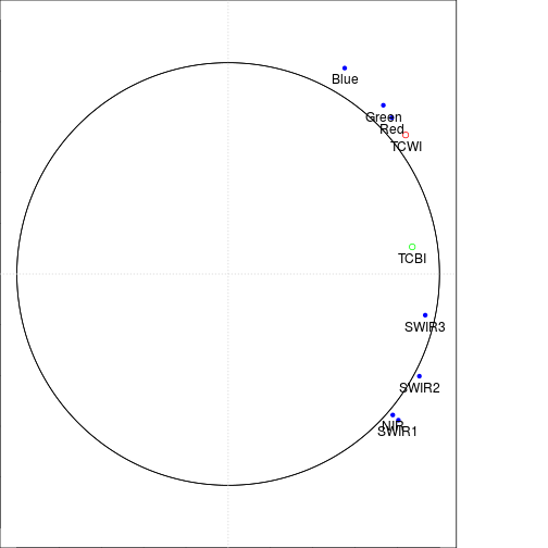
##### Plot on the loading space using TCBI and TCWI as supplementary variables
var_labels <- rownames(loadings_df)

plot(loadings_df[,1],loadings_df[,2],
     type="p",
     pch = 20,
     col ="blue",
     xlab=names(loadings_df)[1],
     ylab=names(loadings_df)[2],
     ylim=c(-1,1),
     xlim=c(-1,1),
     axes = FALSE,
     cex.lab = 1.2)

points(cor_r_TC$pc_scores.1[1],cor_r_TC$pc_scores.2[1],col="red")
points(cor_r_TC$pc_scores.1[2],cor_r_TC$pc_scores.2[2],col="green")

axis(1, at=seq(-1,1,0.2),cex=1.2)
axis(2, las=1,at=seq(-1,1,0.2),cex=1.2) # "1' for side=below, the axis is drawned  on the right at location 0 and 1
box()    #This draws a box...

title(paste0("Loadings for component ", names(loadings_df)[1]," and " ,names(loadings_df)[2] ))
draw.circle(0,0,c(1.0,1.0),nv=500)#,border="purple",
text(loadings_df[,1],loadings_df[,2],var_labels,pos=1,cex=1)
text(cor_r_TC$pc_scores.1[1],cor_r_TC$pc_scores.2[1],"TCWI",pos=1,cex=1)
text(cor_r_TC$pc_scores.1[2],cor_r_TC$pc_scores.2[2],"TCBI",pos=1,cex=1)
grid(2,2)
########################## End of Script ###################################
####################################    Flood Mapping Analyses   #######################################
############################  Analyze and map flooding from RITA hurricane  #######################################
#This script performs analyses for the Exercise 6 of the Short Course using reflectance data derived from MODIS.
#The goal is to map flooding from RITA using various reflectance bands from Remote Sensing platforms.
#Additional data is provided including FEMA flood region.
#
#AUTHORS: Benoit Parmentier
#DATE CREATED: 03/13/2018
#DATE MODIFIED: 04/01/2018
#Version: 1
#PROJECT: SESYNC and AAG 2018 workshop/Short Course preparation
#TO DO:
#
#COMMIT: setting up input data
#
#################################################################################################

###Loading R library and packages

library(sp) # spatial/geographfic objects and functions
library(rgdal) #GDAL/OGR binding for R with functionalities
library(spdep) #spatial analyses operations, functions etc.
library(gtools) # contains mixsort and other useful functions
library(maptools) # tools to manipulate spatial data
library(parallel) # parallel computation, part of base package no
library(rasterVis) # raster visualization operations
library(raster) # raster functionalities
library(forecast) #ARIMA forecasting
library(xts) #extension for time series object and analyses
library(zoo) # time series object and analysis
library(lubridate) # dates functionality
library(colorRamps) #contains matlab.like color palette
library(rgeos) #contains topological operations
library(sphet) #contains spreg, spatial regression modeling
library(BMS) #contains hex2bin and bin2hex, Bayesian methods
library(bitops) # function for bitwise operations
library(foreign) # import datasets from SAS, spss, stata and other sources
#library(gdata) #read xls, dbf etc., not recently updated but useful
library(classInt) #methods to generate class limits
library(plyr) #data wrangling: various operations for splitting, combining data
#library(gstat) #spatial interpolation and kriging methods
library(readxl) #functionalities to read in excel type data
library(psych) #pca/eigenvector decomposition functionalities
library(sf)
library(plotrix) #various graphic functions e.g. draw.circle
library(nnet)
library(rpart)
library(e1071)
Attaching package: 'e1071'
The following object is masked from 'package:raster':

    interpolate
The following object is masked from 'package:gtools':

    permutations
library(caret)
Loading required package: ggplot2
Attaching package: 'ggplot2'
The following objects are masked from 'package:psych':

    %+%, alpha
The following object is masked from 'package:forecast':

    autolayer
The following object is masked from 'package:latticeExtra':

    layer
The following object is masked from 'package:raster':

    calc
###### Functions used in this script

create_dir_fun <- function(outDir,out_suffix=NULL){
  #if out_suffix is not null then append out_suffix string
  if(!is.null(out_suffix)){
    out_name <- paste("output_",out_suffix,sep="")
    outDir <- file.path(outDir,out_name)
  }
  #create if does not exists
  if(!file.exists(outDir)){
    dir.create(outDir)
  }
  return(outDir)
}

#Used to load RData object saved within the functions produced.
load_obj <- function(f){
  env <- new.env()
  nm <- load(f, env)[1]
  env[[nm]]
}

#####  Parameters and argument set up ###########

in_dir_var <- "../data"
out_dir <- "."

#region coordinate reference system
#http://spatialreference.org/ref/epsg/nad83-texas-state-mapping-system/proj4/
CRS_reg <- "+proj=lcc +lat_1=27.41666666666667 +lat_2=34.91666666666666 +lat_0=31.16666666666667 +lon_0=-100 +x_0=1000000 +y_0=1000000 +ellps=GRS80 +datum=NAD83 +units=m +no_defs"
file_format <- ".tif" #PARAM5
NA_flag_val <- -9999 #PARAM6
out_suffix <-"exercise6_03312018" #output suffix for the files and ouptu folder #PARAM 8
create_out_dir_param=TRUE #PARAM9

#ARG9
#local raster name defining resolution, extent
infile_RITA_reflectance_date2 <- "mosaiced_MOD09A1_A2005273__006_reflectance_masked_RITA_reg_1km.tif"
infile_reg_outline <- "new_strata_rita_10282017" # Region outline and FEMA zones
infile_modis_bands_information <- "df_modis_band_info.txt" # MOD09 bands information.
nlcd_2006_filename <- "nlcd_2006_RITA.tif" # NLCD2006 Land cover data aggregated at ~ 1km.

###########################  START SCRIPT  ##############################

####### SET UP OUTPUT DIRECTORY #######

## First create an output directory

if(is.null(out_dir)){
  out_dir <- dirname(in_dir) #output will be created in the input dir
}

out_suffix_s <- out_suffix #can modify name of output suffix
if(create_out_dir_param==TRUE){
  out_dir <- create_dir_fun(out_dir,out_suffix_s)
  setwd(out_dir)
}else{
  setwd(out_dir) #use previoulsy defined directory
}

#####################################
##### PART I: DISPLAY AND EXPLORE DATA ##############

#### MOD09 raster image after hurricane Rita
r_after <- brick(file.path(in_dir_var,infile_RITA_reflectance_date2))

## Read band information since it is more informative!!
df_modis_band_info <- read.table(file.path(in_dir_var,infile_modis_bands_information),
                                 sep=",",
                                 stringsAsFactors = F)
print(df_modis_band_info)
  band_name band_number start_wlength end_wlength
1       Red           3           620         670
2       NIR           4           841         876
3      Blue           1           459         479
4     Green           2           545         565
5     SWIR1           5          1230        1250
6     SWIR2           6          1628        1652
7     SWIR3           7          2105        2155
df_modis_band_info$band_number <- c(3,4,1,2,5,6,7)
write.table(df_modis_band_info,file.path(in_dir_var,infile_modis_bands_information),
            sep=",")

band_refl_order <- df_modis_band_info$band_number

names(r_after) <- df_modis_band_info$band_name

## Use subset instead of $ if you want to wrap code into function
r_after_MNDWI <- (subset(r_after,"Green") - subset(r_after,"SWIR2")) / (subset(r_after,"Green") + subset(r_after,"SWIR2"))
plot(r_after_MNDWI,zlim=c(-1,1))
r_after_NDVI <- (subset(r_after,"NIR") - subset(r_after,"Red")) / (subset(r_after,"NIR") + subset(r_after,"Red"))
plot(r_after_NDVI)
data_type_str <- dataType(r_after_NDVI)

NAvalue(r_after_NDVI) <- NA_flag_val
out_filename <- paste("ndvi_post_Rita","_",out_suffix,file_format,sep="")
out_filename <- file.path(out_dir,out_filename)
writeRaster(r_after_NDVI,
            filename=out_filename,
            datatype=data_type_str,
            overwrite=T)
Error in .local(x, filename, ...): Attempting to write a file to a path that does not exist:
  ./output_exercise6_03312018
NAvalue(r_after_MNDWI) <- NA_flag_val
out_filename <- paste("mndwi_post_Rita","_",out_suffix,file_format,sep="")
out_filename <- file.path(out_dir,out_filename)
writeRaster(r_after_MNDWI,
            filename=out_filename,
            datatype=data_type_str,
            overwrite=T)
Error in .local(x, filename, ...): Attempting to write a file to a path that does not exist:
  ./output_exercise6_03312018
#training_data_sf <- st_read("training1.shp")
#1) vegetation and other (small water fraction)
#2) Flooded vegetation
#3) Flooded area, or water (lake etc)

class1_data_sf <- st_read(file.path(in_dir_var,"class1_sites"))
Reading layer `class1_sites' from data source `/nfs/public-data/training/class1_sites' using driver `ESRI Shapefile'
Simple feature collection with 6 features and 2 fields
geometry type:  POLYGON
dimension:      XY
bbox:           xmin: 1588619 ymin: 859495.9 xmax: 1830803 ymax: 941484.1
epsg (SRID):    NA
proj4string:    NA
class2_data_sf <- st_read(file.path(in_dir_var,"class2_sites"))
Reading layer `class2_sites' from data source `/nfs/public-data/training/class2_sites' using driver `ESRI Shapefile'
Simple feature collection with 8 features and 2 fields
geometry type:  MULTIPOLYGON
dimension:      XY
bbox:           xmin: 1605433 ymin: 848843.8 xmax: 1794265 ymax: 884027.8
epsg (SRID):    NA
proj4string:    NA
class3_data_sf <- st_read(file.path(in_dir_var,"class3_sites"))
Reading layer `class3_sites' from data source `/nfs/public-data/training/class3_sites' using driver `ESRI Shapefile'
Simple feature collection with 9 features and 2 fields
geometry type:  POLYGON
dimension:      XY
bbox:           xmin: 1587649 ymin: 845271.3 xmax: 1777404 ymax: 891073.1
epsg (SRID):    NA
proj4string:    NA
### combine object, note they should be in the same projection system
class_data_sf <- rbind(class1_data_sf,class2_data_sf,class3_data_sf)
class_data_sf$poly_ID <- 1:nrow(class_data_sf) #unique ID for each polygon
nrow(class_data_sf) # 23 different polygons used at ground truth data
[1] 23
class_data_sp <- as(class_data_sf,"Spatial")

r_x <- init(r_after,"x") #raster with coordinates x
r_y <- init(r_after,"x") #raster with coordiates y

r_stack <- stack(r_x,r_y,r_after,r_after_NDVI,r_after_MNDWI)
names(r_stack) <- c("x","y","Red","NIR","Blue","Green","SWIR1","SWIR2","SWIR3","NDVI","MNDWI")
pixels_extracted_df <- extract(r_stack,class_data_sp,df=T)
Warning in merge.data.frame(as.data.frame(x), as.data.frame(y), ...):
column name 'x' is duplicated in the result

Warning in merge.data.frame(as.data.frame(x), as.data.frame(y), ...):
column name 'x' is duplicated in the result

Warning in merge.data.frame(as.data.frame(x), as.data.frame(y), ...):
column name 'x' is duplicated in the result

Warning in merge.data.frame(as.data.frame(x), as.data.frame(y), ...):
column name 'x' is duplicated in the result

Warning in merge.data.frame(as.data.frame(x), as.data.frame(y), ...):
column name 'x' is duplicated in the result

Warning in merge.data.frame(as.data.frame(x), as.data.frame(y), ...):
column name 'x' is duplicated in the result

Warning in merge.data.frame(as.data.frame(x), as.data.frame(y), ...):
column name 'x' is duplicated in the result

Warning in merge.data.frame(as.data.frame(x), as.data.frame(y), ...):
column name 'x' is duplicated in the result

Warning in merge.data.frame(as.data.frame(x), as.data.frame(y), ...):
column name 'x' is duplicated in the result

Warning in merge.data.frame(as.data.frame(x), as.data.frame(y), ...):
column name 'x' is duplicated in the result

Warning in merge.data.frame(as.data.frame(x), as.data.frame(y), ...):
column name 'x' is duplicated in the result

Warning in merge.data.frame(as.data.frame(x), as.data.frame(y), ...):
column name 'x' is duplicated in the result

Warning in merge.data.frame(as.data.frame(x), as.data.frame(y), ...):
column name 'x' is duplicated in the result

Warning in merge.data.frame(as.data.frame(x), as.data.frame(y), ...):
column name 'x' is duplicated in the result

Warning in merge.data.frame(as.data.frame(x), as.data.frame(y), ...):
column name 'x' is duplicated in the result

Warning in merge.data.frame(as.data.frame(x), as.data.frame(y), ...):
column name 'x' is duplicated in the result

Warning in merge.data.frame(as.data.frame(x), as.data.frame(y), ...):
column name 'x' is duplicated in the result

Warning in merge.data.frame(as.data.frame(x), as.data.frame(y), ...):
column name 'x' is duplicated in the result

Warning in merge.data.frame(as.data.frame(x), as.data.frame(y), ...):
column name 'x' is duplicated in the result

Warning in merge.data.frame(as.data.frame(x), as.data.frame(y), ...):
column name 'x' is duplicated in the result

Warning in merge.data.frame(as.data.frame(x), as.data.frame(y), ...):
column name 'x' is duplicated in the result

Warning in merge.data.frame(as.data.frame(x), as.data.frame(y), ...):
column name 'x' is duplicated in the result

Warning in merge.data.frame(as.data.frame(x), as.data.frame(y), ...):
column name 'x' is duplicated in the result
dim(pixels_extracted_df) #We have 1547 pixels extracted
[1] 1547 12
class_data_df <- class_data_sf
st_geometry(class_data_df) <- NULL #this will coerce the sf object into a data.frame

pixels_df <- merge(pixels_extracted_df,class_data_df,by.x="ID",by.y="poly_ID")

head(pixels_df)
  ID       x       y        Red       NIR       Blue      Green     SWIR1
1  1 1615340 1615340 0.05304649 0.3035397 0.02652384 0.05662384 0.3101271
2  1 1614413 1614413 0.05782417 0.3295924 0.02751791 0.06305390 0.3453724
3  1 1615340 1615340 0.05735013 0.3037102 0.02596963 0.05654212 0.3176476
4  1 1616266 1616266 0.05805403 0.3081988 0.02711912 0.05750944 0.3229090
5  1 1617193 1617193 0.04147716 0.3058677 0.01839499 0.05076184 0.3003513
6  1 1618120 1618120 0.04209801 0.3089238 0.01832494 0.05200353 0.2943777
      SWIR2      SWIR3      NDVI      MNDWI record_ID class_ID
1 0.1936452 0.07864757 0.7024759 -0.5474962         1        1
2 0.2102322 0.08679578 0.7014884 -0.5385502         1        1
3 0.2073480 0.08732812 0.6823238 -0.5714722         1        1
4 0.2079238 0.08741243 0.6829839 -0.5666749         1        1
5 0.1692552 0.06590501 0.7611759 -0.5385644         1        1
6 0.1697936 0.06790353 0.7601402 -0.5310712         1        1
table(pixels_df$class_ID) # count by class of pixels ground truth data
  1   2   3
508 285 754
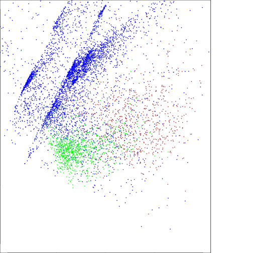
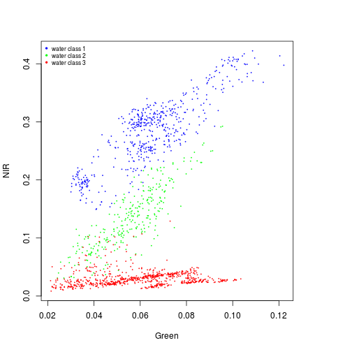
######## Examining sites data used for the classification

#Water
x_range <- range(pixels_df$Green,na.rm=T)
y_range <- range(pixels_df$NIR,na.rm=T)

###Add legend?
plot(NIR~Green,xlim=x_range,ylim=y_range,cex=0.2,col="blue",subset(pixels_df,class_ID==1))
points(NIR~Green,col="green",cex=0.2,subset(pixels_df,class_ID==2))
points(NIR~Green,col="red",cex=0.2,subset(pixels_df,class_ID==3))
names_vals <- c("water class 1","water class 2","water class 3")
legend("topleft",legend=names_vals,
       pt.cex=0.7,cex=0.7,col=c("blue","green","red"),
       pch=20, #add circle symbol to line
       bty="n")
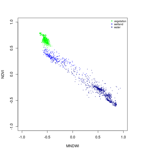
## Let's use a palette that reflects wetness or level of water
col_palette <- c("green","blue","darkblue")
plot(NDVI ~ MNDWI,
xlim=c(-1,1),ylim=c(-1,1),
cex=0.2,
col=col_palette[1],
subset(pixels_df,class_ID==1))
points(NDVI ~ MNDWI,
cex=0.2,
col=col_palette[2],
subset(pixels_df,class_ID==2))
points(NDVI ~ MNDWI,
cex=0.2,
col=col_palette[3],
subset(pixels_df,class_ID==3))
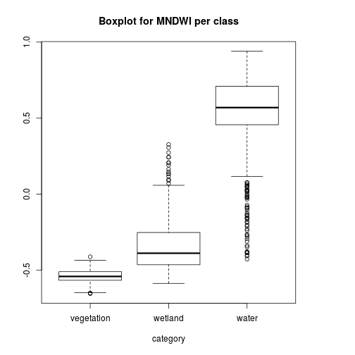
names_vals <- c("vegetation","wetland","water")
legend("topright",legend=names_vals,
pt.cex=0.7,cex=0.7,col=col_palette,
pch=20, #add circle symbol to line
bty="n")
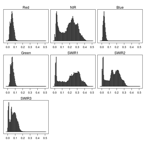
histogram(r_after)
pixels_df$class_ID <- factor(pixels_df$class_ID,
                    levels = c(1,2,3),
                    labels = names_vals)

boxplot(MNDWI~class_ID,
        pixels_df,
        xlab="category",
        main="Boxplot for MNDWI per class")
###############################################
##### PART II: Split training and testing ##############

##let's keep 30% of data for testing for each class

pixels_df$pix_ID <- 1:nrow(pixels_df)
prop <- 0.3
table(pixels_df$class_ID)
vegetation    wetland      water
       508        285        754
set.seed(100) ## set random seed for reproducibility

### This is for one class:
##Better as a function but we use a loop for clarity here:

list_data_df <- vector("list",length=3)
level_labels <- names_vals

for(i in 1:3){
  data_df <- subset(pixels_df,class_ID==level_labels[i])
  data_df$pix_id <- 1:nrow(data_df)
  indices <- as.vector(createDataPartition(data_df$pix_ID,p=0.7,list=F))
  data_df$training <-  as.numeric(data_df$pix_id %in% indices)
  list_data_df[[i]] <- data_df
}

data_df <- do.call(rbind,list_data_df)

dim(data_df)
[1] 1547 17
head(data_df)
  ID       x       y        Red       NIR       Blue      Green     SWIR1
1  1 1615340 1615340 0.05304649 0.3035397 0.02652384 0.05662384 0.3101271
2  1 1614413 1614413 0.05782417 0.3295924 0.02751791 0.06305390 0.3453724
3  1 1615340 1615340 0.05735013 0.3037102 0.02596963 0.05654212 0.3176476
4  1 1616266 1616266 0.05805403 0.3081988 0.02711912 0.05750944 0.3229090
5  1 1617193 1617193 0.04147716 0.3058677 0.01839499 0.05076184 0.3003513
6  1 1618120 1618120 0.04209801 0.3089238 0.01832494 0.05200353 0.2943777
      SWIR2      SWIR3      NDVI      MNDWI record_ID   class_ID pix_ID
1 0.1936452 0.07864757 0.7024759 -0.5474962         1 vegetation      1
2 0.2102322 0.08679578 0.7014884 -0.5385502         1 vegetation      2
3 0.2073480 0.08732812 0.6823238 -0.5714722         1 vegetation      3
4 0.2079238 0.08741243 0.6829839 -0.5666749         1 vegetation      4
5 0.1692552 0.06590501 0.7611759 -0.5385644         1 vegetation      5
6 0.1697936 0.06790353 0.7601402 -0.5310712         1 vegetation      6
  pix_id training
1      1        0
2      2        1
3      3        0
4      4        0
5      5        1
6      6        0
data_training <- subset(data_df,training==1)
###############################################
##### PART III: Generate classification using CART and SVM ##############
############### Using Classification and Regression Tree model (CART) #########
## Fit model using training data for CART
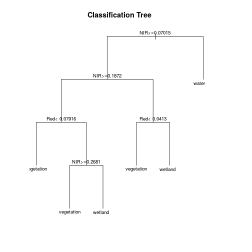
mod_rpart <- rpart(class_ID ~ Red + NIR + Blue + Green + SWIR1 + SWIR2 + SWIR3,
method="class",
data=data_training)
# Plot the fitted classification tree
plot(mod_rpart, uniform=TRUE, main="Classification Tree")
text(mod_rpart, cex=.8)
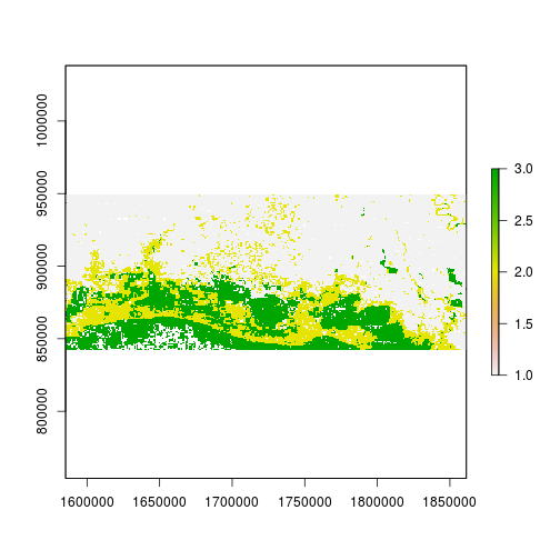
# Now predict the subset data based on the model; prediction for entire area takes longer time
raster_out_filename <- paste0("r_predicted_rpart_",out_suffix,file_format)
r_predicted_rpart <- predict(r_stack,mod_rpart,
                             type='class',
                             filename=raster_out_filename,
                             progress = 'text',
                             overwrite=T)
  |
  |                                                                 |   0%
  |
  |================                                                 |  25%
  |
  |================================                                 |  50%
  |
  |=================================================                |  75%
  |
  |=================================================================| 100%
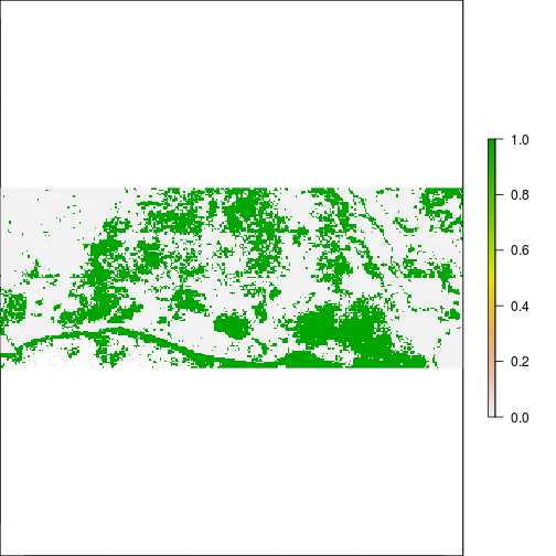
plot(r_predicted_rpart)
r_predicted_rpart <- ratify(r_predicted_rpart)
rat <- levels(r_predicted_rpart)[[1]]
rat$legend <- c("vegetation","wetland","water")
levels(r_predicted_rpart) <- rat
levelplot(r_predicted_rpart, maxpixels = 1e6,
          col.regions = c("green","blue","darkblue"),
          scales=list(draw=FALSE),
          main = "Classification Tree")

############### Using Support Vector Machine #########

## set class_ID as factor to generate classification

mod_svm <- svm(class_ID ~ Red +NIR + Blue + Green + SWIR1 + SWIR2 + SWIR3,
               data=data_training,
               method="C-classification",
               kernel="linear") # can be radial

summary(mod_svm)
Call:
svm(formula = class_ID ~ Red + NIR + Blue + Green + SWIR1 + SWIR2 +
    SWIR3, data = data_training, method = "C-classification",
    kernel = "linear")


Parameters:
   SVM-Type:  C-classification
 SVM-Kernel:  linear
       cost:  1
      gamma:  0.1428571

Number of Support Vectors:  110

 ( 12 54 44 )


Number of Classes:  3

Levels:
 vegetation wetland water
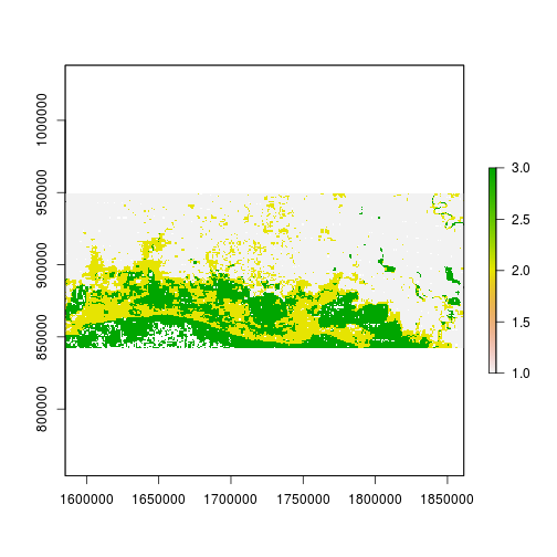
# Now predict the subset data based on the model; prediction for entire area takes longer time
raster_outfilename <- paste0("r_predicted_svm_",out_suffix,file_format)
r_predicted_svm <- predict(r_stack, mod_svm,
                           progress = 'text',
                           filename=raster_outfilename,
                           overwrite=T)
  |
  |                                                                 |   0%
  |
  |================                                                 |  25%
  |
  |================================                                 |  50%
  |
  |=================================================                |  75%
  |
  |=================================================================| 100%
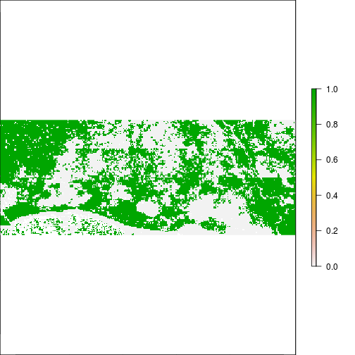
plot(r_predicted_svm)
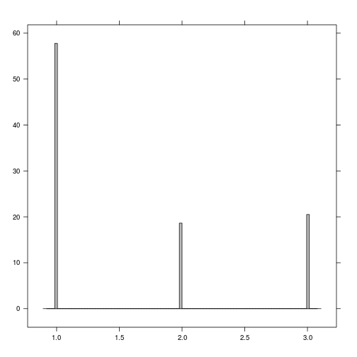
histogram(r_predicted_svm)
r_predicted_svm <- ratify(r_predicted_svm)
rat <- levels(r_predicted_svm)[[1]]
rat$legend <- c("vegetation","wetland","water")
levels(r_predicted_svm) <- rat
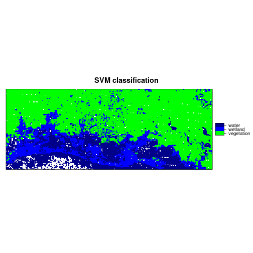
levelplot(r_predicted_svm, maxpixels = 1e6,
col.regions = c("green","blue","darkblue"),
scales=list(draw=FALSE),
main = "SVM classification")
###############################################
##### PART IV: Compare methods for the performance ##############

dim(data_df) # full dataset, let's use data points for testing
[1] 1547 17
#omit values that contain NA, because may be problematic with SVM.
data_testing <- na.omit(subset(data_df,training==0))
dim(data_testing)
[1] 450 17
#### Predict on testing data using rpart model fitted with training data
testing_rpart <- predict(mod_rpart, data_testing,type='class')
#### Predict on testing data using SVM model fitted with training data
testing_svm <- predict(mod_svm,data_testing, type='class')

## Predicted classes:
table(testing_svm)
testing_svm
vegetation    wetland      water
       150         78        222
#### Generate confusion matrix to assess the performance of the model

tb_rpart <- table(testing_rpart,data_testing$class_ID)
tb_svm <- table(testing_svm,data_testing$class_ID)

#testing_rpart: map prediction in the rows
#data_test$class_ID: ground truth data in the columns
#http://spatial-analyst.net/ILWIS/htm/ilwismen/confusion_matrix.htm
#Producer accuracy: it is the fraction of correctly classified pixels with regard to all pixels
#of that ground truth class.

table(testing_rpart) #classification, map results
testing_rpart
vegetation    wetland      water
       149         77        224
table(data_testing$class_ID) #reference, ground truth in columns
vegetation    wetland      water
       149         84        217
tb_rpart[1]/sum(tb_rpart[,1]) #producer accuracy
[1] 0.9798658
tb_svm[1]/sum(tb_svm[,1]) #producer accuracy
[1] 1
#overall accuracy for svm
sum(diag(tb_svm))/sum(table(testing_svm))
[1] 0.9644444
#overall accuracy for rpart
sum(diag(tb_rpart))/sum(table(testing_rpart))
[1] 0.9444444
#Generate more accuracy measurements from CARET
accuracy_info_svm <- confusionMatrix(testing_svm,data_testing$class_ID, positive = NULL)
accuracy_info_rpart <- confusionMatrix(testing_rpart,data_testing$class_ID, positive = NULL)

accuracy_info_rpart$overall
      Accuracy          Kappa  AccuracyLower  AccuracyUpper   AccuracyNull
  9.444444e-01   9.101603e-01   9.190787e-01   9.637284e-01   4.822222e-01
AccuracyPValue  McnemarPValue
 1.266887e-101            NaN
accuracy_info_svm$overall
      Accuracy          Kappa  AccuracyLower  AccuracyUpper   AccuracyNull
  9.644444e-01   9.425947e-01   9.429011e-01   9.795429e-01   4.822222e-01
AccuracyPValue  McnemarPValue
 9.645095e-114            NaN
#### write out the results:
write.table(accuracy_info_rpart$table,"confusion_matrix_rpart.txt",sep=",")
write.table(accuracy_info_svm$table,"confusion_matrix_svm.txt",sep=",")

############################ End of Script ###################################