Database Principles and Use
Note: This lesson is in beta status! It may have issues that have not been addressed.
Handouts for this lesson need to be saved on your computer. Download and unzip this material into the directory (a.k.a. folder) where you plan to work.
What good is a database?
For a team of researchers implementing a collaborative workflow, the top three reasons to use a database are:
- concurrency - Multiple users can safely read and edit database entries simultaneously.
- reliability - Relational databases formalize and can enforce concepts of “tidy” data.
- scalability - Very large tables can be read, searched, and merged quickly.
In this lesson, the term “database” more precisely means a relational database that allows data manipulation with Structured Query Language (SQL). Strictly speaking, the word “database” describes any collection of digitized data–a distinction that has mostly outlived its usefulness.
Objectives
- Understand how a database differs from a data file
- Introduce the SQLite database system
- Meet Structured Query Language (SQL)
- Recognize the value of typed data
Specific Achievements
- Access a SQLite database from RStudio
- Create a table and view table definitions
- Insert records one at a time into a table
- Check primary and foreign key constraints
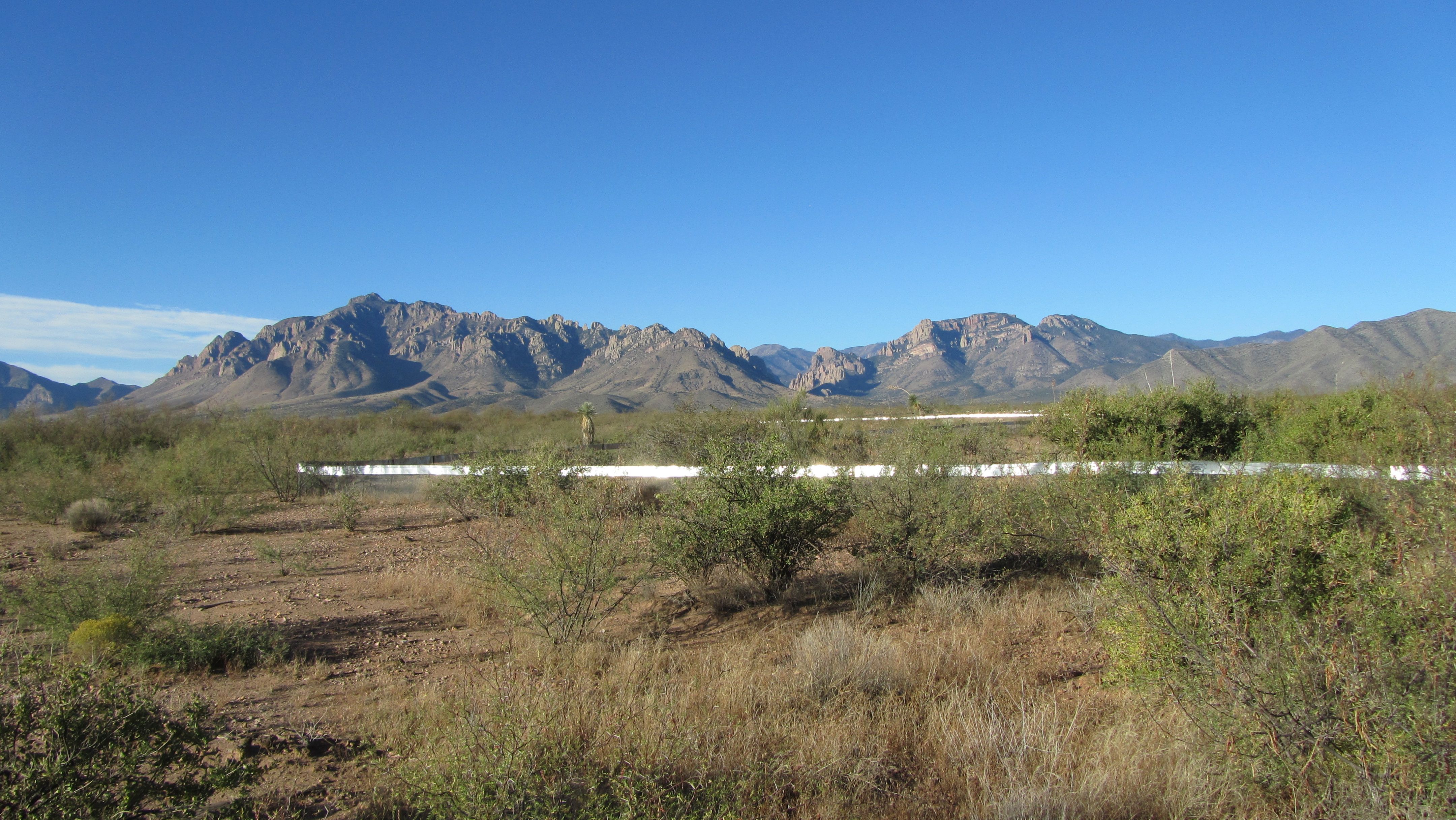
The Portal Project

Credit: The Portal Project
The Portal Project is a long-term ecological study being conducted near Portal, AZ. Since 1977, the site has been a primary focus of research on interactions among rodents, ants and plants and their respective responses to climate.
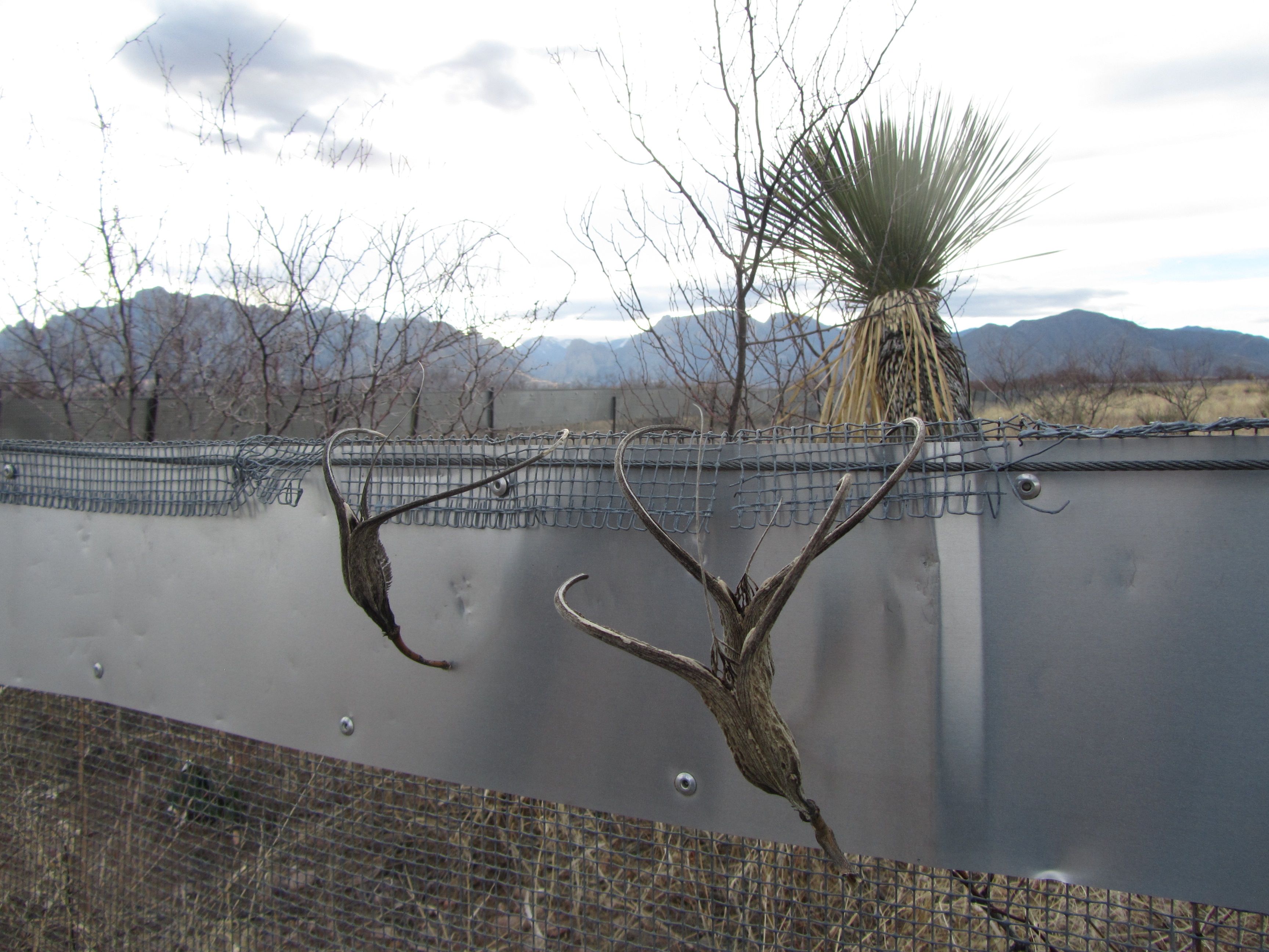
Credit: The Portal Project
The research site consists of many plots – patches of the Arizona desert that are intensively manipulated and repeatedly surveyed. The plots have some fixed characteristics, such as the type of manipulation, geographic location, aspect, etc.
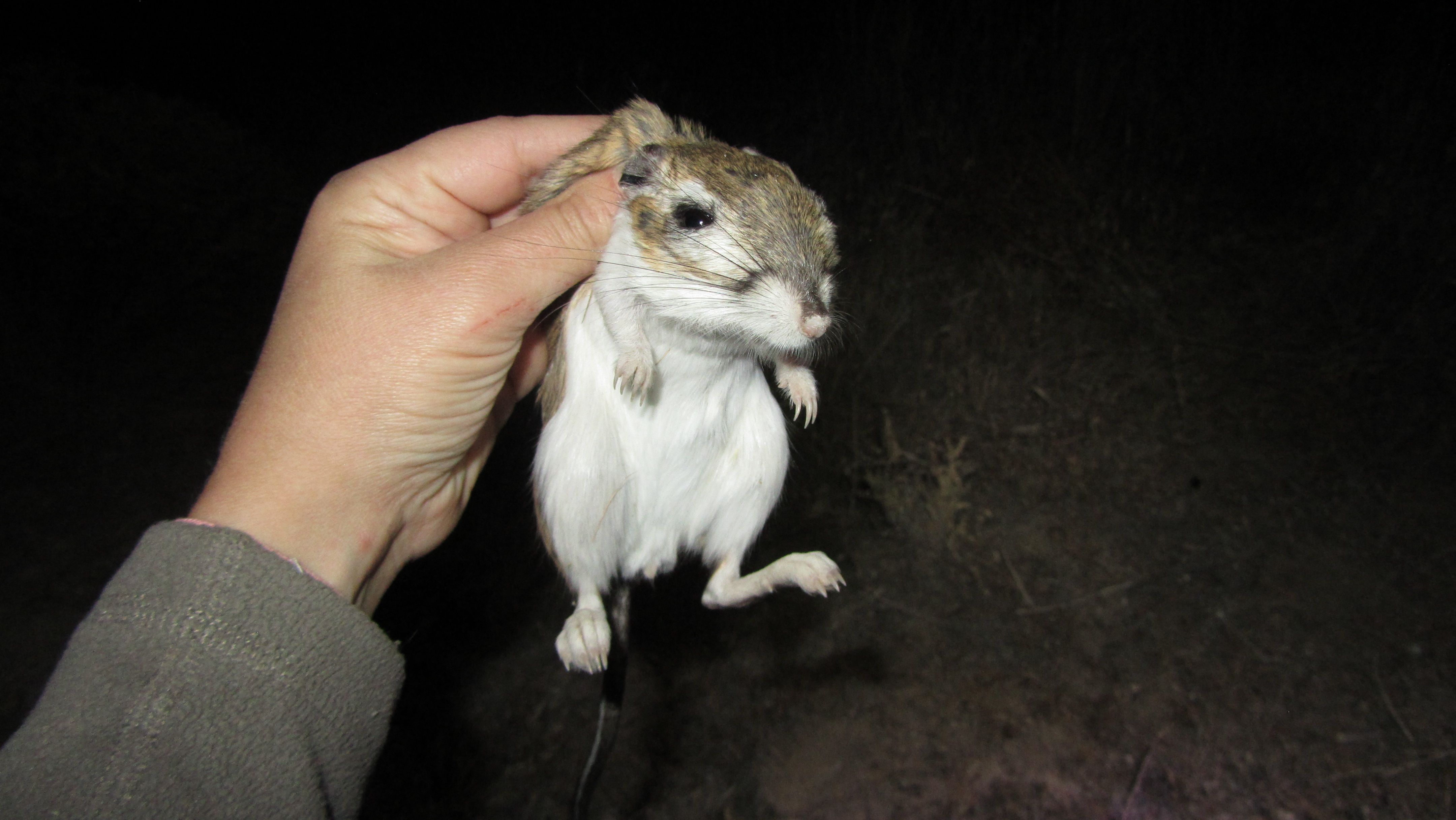
Credit: The Portal Project
The plots have a lot of dynamic characteristics, and those changes are recorded in repeated surveys. In particular, the animals captured during each survey are identified to species, weighed, and measured.
Credit: The Portal Project
Data from the Portal project is recorded in a relational database designed for reliable storage & rapid access to the bounty of information produced by this long-term ecological experiment.
This lesson uses real data, which has been analyzed in over 100 publications. The data been simplified just a little bit for the workshop, but you can download the full dataset and work with it using exactly the same tools we learn today.
The three key tables in the relational database are:
- plots
- surveys
- species
Database Characteristics: I
Database terminology builds on common ways of characterizing data files. The breakdown of a table into records (by row) or fields (by column) is familiar to anyone who’s worked in spreadsheets. The descriptions below formalize these terms, and provide an example referencing the Portal mammals database.
| Field | The smallest unit of information, each having a label and holding a value of the same type. e.g. The day on which a plot was surveyed. |
| Record | A collection of related values, from different fields, that all describe the same entity. e.g. The species, sex, weight and size of a small mammal captured during a survey. |
| Table | A collection of records, each one uniquely identified by the value of a key field. e.g. All records for small mammals observed during any survey. |
Software for using a database provides different tools for working with tables than a spreadsheet program. A database is generally characterized as being tooled for production environments, in contrast to data files tooled for ease of use.
Collaboration
- Data files are stored in the cloud (sync issues), shared on a network (user collision), or copies are emailed among collaborators.
- A database server accepts simultaneous users from different clients on a network. There are never multiple copies of the data (aside from backups!).
SQLite databases are not directly comparable to client/server database systems because they store data locally. Although this can provide greater simplicity and ease of use, it may require more coordination among collaborators.
Size
- Reading an entire data file into memory isn’t scaleable. Some file types (e.g. MS Excel files) have size limits.
- Database software only reads requested parts of the data into memory. There are no size limits.
Quality
- Data file formats do not typically provide any quality controls.
- Databases stricly enforce data types on each field. Letters, for example “N.A.”, cannot be entered into a field for integers.
Extension
- Specialized files are needed for complicated data types (e.g. ESRI Shapefiles).
- Databases provide many non-standard data types, and very specialized ones (e.g. geometries, time and date) are available through extension packages.
Programming
- There is no standard way to read, edit, or create records in data files of different formats or from different languages.
- Packages native to all popular programming languages provide access to databases using SQL.
Connecting to a Database
We are going to look at the Portal mammals data organized in an SQLite database.
This is stored in a single file portal.sqlite that can be explored using SQL
or with tools like SQLite Viewer or DB Browser. We will use R functions in the DBI-compliant
RSQLite package to interact with the database.
Connections
The first step from RStudio is creating a connection object that opens up a channel of communication to the database file.
library(RSQLite)
con <- dbConnect(RSQLite::SQLite(),
                 "data/portal.sqlite")
With the connection object availble, you can begin exploring the database.
> dbListTables(con)
[1] "observers" "plots" "species" "surveys"
> dbListFields(con, 'species')
[1] "species_id" "genus" "species" "taxa"
Read an entire database table into an R data frame with dbReadTable, or if you
prefer “tidyverse” functions, use the dplyr tbl function.
library(dplyr)
species <- tbl(con, 'species')
> species
# Source:   table<species> [?? x 4]
# Database: sqlite 3.36.0 [/nfs/public-data/training/portal.sqlite]
   species_id genus            species         taxa
   <chr>      <chr>            <chr>           <chr>
 1 AB         Amphispiza       bilineata       Bird
 2 AH         Ammospermophilus harrisi         Rodent
 3 AS         Ammodramus       savannarum      Bird
 4 BA         Baiomys          taylori         Rodent
 5 CB         Campylorhynchus  brunneicapillus Bird
 6 CM         Calamospiza      melanocorys     Bird
 7 CQ         Callipepla       squamata        Bird
 8 CS         Crotalus         scutalatus      Reptile
 9 CT         Cnemidophorus    tigris          Reptile
10 CU         Cnemidophorus    uniparens       Reptile
# … with more rows
The dbWriteTable function provides a mechanism for uploading data, as long as
the user specified in the connection object has permission to create tables.
df <- data.frame(
  id = c(1, 2),
  name = c('Alice', 'Bob')
)

dbWriteTable(con, "observers",
             value = df, overwrite = TRUE)
> dbReadTable(con, 'observers')
Database Characteristics: II
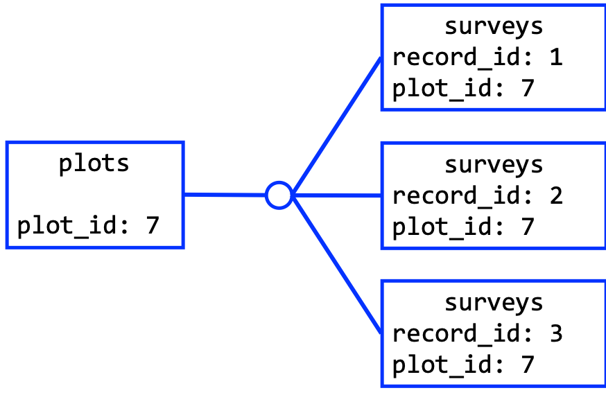
Returning to the bigger picture and our comparison of storing data in files as opposed to a database, there are some concepts that only apply to databases. We have seen that databases include multiple tables—so far, that’s not so different from keeping multiple spreadsheets in one MS Excel workbook or in multiple CSV files. The collection of tables in a relational database, however, can be structured by built-in relationships between records from different tables. Data is assembled in the correct arrangement for analysis “just in time” by scripting database queries that join tables on these relationships.
| Primary key | One or more fields (but usually one) that uniquely identify a record in a table. |
| Foreign key | A primary key from one table used in different table to establish a relationship. |
| Query | Collect values from tables based on their relationships and other constraints. |
Primary Keys
In the plots table, id is the primary key. Any new record cannot duplicate an existing id.
| id | treatment |
|---|---|
| 1 | Control |
| 2 | Rodent Exclosure |
| 3 | Control |
Recreate the observers table with id as a primary key; this will prevent the
duplication observed from multiple identical dbWriteTable calls.
dbRemoveTable(con, 'observers') # remove the old version of the table

# create the new version of the table
dbCreateTable(con, 'observers', list(
  id = 'integer primary key',
  name = 'text', overwrite = TRUE
))
When appending a data frame to the table created with “integer primary key”,
the id is automatically generated and unique.
df <- data.frame(
  name = c('Alice', 'Bob')
)
dbWriteTable(con, 'observers', df,
             append = TRUE)
Primary keys are checked before duplicates end up in the data, throwing an error if necessary.
df <- data.frame(
  id = c(1),
  name = c('J. Doe')
)
dbWriteTable(con, 'observers', df,
             append = TRUE)
Error: UNIQUE constraint failed: observers.id
Foreign Keys
A field may also be designated as a foreign key, which establishes a relationship between tables. A foreign key points to some primary key from a different table.
In the surveys table, id is the primary key and both plot_id and
species_id are foreign keys.
| id | month | day | year | plot_id | species_id | sex | hindfoot_length | weight |
|---|---|---|---|---|---|---|---|---|
| 1 | 7 | 16 | 1977 | 2 | ST | M | 32 | 0.45 |
| 2 | 7 | 16 | 1977 | 2 | PX | M | 33 | 0.23 |
| 3 | 7 | 16 | 1978 | 1 | RO | F | 14 | 1.23 |
To enable foreign key constraints in sqlite run the following:
dbExecute(con, 'PRAGMA foreign_keys = ON;')
[1] 0
Foreign keys are checked before nonsensical references end up in the data. To enable foreign key constraints in sqlite run the following:
df <- data.frame(
  month = 7,
  day = 16,
  year = 1977,
  plot_id = 'Rodent'
)
dbWriteTable(con, 'surveys', df,
             append = TRUE)
Error: FOREIGN KEY constraint failed
Query
Structured Query Language (SQL) is a high-level language for interacting with relational databases. Commands use intuitive English words but can be strung together and nested in powerful ways. SQL is not the only way to query a database from R (cf. dbplyr), but sometimes it is the only way to perform a complicated query.
To write SQL statements in RStudio, it is also possible to use the sql engine for code chunks in a
RMarkdown file:
`
``{sql connection = con}
...
`
``
We will continue to use R functions to pass SQL code to the database file using dbGetQuery functions.
Basic queries
Let’s write a SQL query that selects only the year column from the animals table.
dbGetQuery(con, "SELECT year FROM surveys")
A note on style: we have capitalized the words SELECT and FROM because they are SQL keywords. Unlike R, SQL is case insensitive, so capitalization only helps for readability and is a good style to adopt.
To select data from multiple fields, include multiple fields as a comma-separated list right after SELECT:
dbGetQuery(con, "SELECT year, month, day
           FROM surveys")
The line break before FROM is also good form, particularly as the length of the query grows.
Or select all of the columns in a table using a wildcard:
dbGetQuery(con, "SELECT *
FROM surveys")
Limit
We can use the LIMIT statement to select only the first few rows. This is particularly helpful when getting a feel for very large tables.
dbGetQuery(con, "SELECT year, species_id
FROM surveys
LIMIT 4")
Unique values
If we want only the unique values so that we can quickly see what species have
been sampled we use DISTINCT
dbGetQuery(con, "SELECT DISTINCT species_id
FROM surveys")
If we select more than one column, then the distinct pairs of values are returned
dbGetQuery(con, "SELECT DISTINCT year, species_id
FROM surveys")
Calculations
We can also do calculations with the values in a query. For example, if we wanted to look at the mass of each individual, by plot, species, and sex, but we needed it in kg instead of g we would use
dbGetQuery(con, "SELECT plot_id, species_id,
  sex, weight / 1000.0
FROM surveys")
The expression weight / 1000.0 is evaluated for each row
and appended to that row, in a new column.
You can assign the new column a name by typing “AS weight_kg” after the expression.
dbGetQuery(con, "SELECT plot_id, species_id, sex,
  weight / 1000 AS weight_kg
FROM surveys")
Expressions can use any fields, any arithmetic operators (+ - * /) and a variety of built-in functions. For example, we could round the values to make them easier to read.
dbGetQuery(con, "SELECT plot_id, species_id, sex,
  ROUND(weight / 1000.0, 2) AS weight_kg
FROM surveys")
The underlying data in the wgt column of the table does not change. The query, which exists separately from the data, simply displays the calculation we requested in the query result window pane.
Filtering
Databases can also filter data – selecting only those records meeting certain
criteria. For example, let’s say we only want data for the species “Dipodomys
merriami”, which has a species code of “DM”. We need to add a WHERE clause to
our query.
dbGetQuery(con, "SELECT *
FROM surveys
WHERE species_id = 'DM'")
Of course, we can do the same thing with numbers.
dbGetQuery(con, "SELECT *
FROM surveys
WHERE year >= 2000")
More sophisticated conditions arise from combining tests with AND and OR. For example, suppose we want the data on Dipodomys merriami starting in the year 2000.
dbGetQuery(con, "SELECT *
FROM surveys
WHERE year >= 2000 AND species_id = 'DM'")
Parentheses can be used to help with readability and to ensure that AND and OR are combined in the way that we intend. If we wanted to get all the animals for “DM” since 2000 or up to 1990 we could combine the tests using OR:
dbGetQuery(con, "SELECT *
FROM surveys
WHERE (year >= 2000 OR year <= 1990)
  AND species_id = 'DM'")
Normalized Data is Tidy
Proper use of table relationships is a challenging part of database design. The objective is normalization, or taking steps to define logical “observational units” and minimize data redundency.
For example, the genus and species names are not attributes of an animal: they are attributes of the species attributed to an animal. Data about a species belongs in a different observational unit from data about the animal captured in a survey. With an ideal database design, any value discovered to be erroneous should only have to be corrected in one record in one table.
- Question
- Currently,
plotsis pretty sparse. What other kind of data might go into plots? - Answer
- Additional properties, such as location, that do not change between surveys.
Un-tidy data with JOINs
A good data management principle is to record and store data in the most normalized form possible, and un-tidy your tables as needed for particular analyses. The SQL “JOIN” clause lets you create records with fields from multiple tables.
Consider for example what you must do to carry out a regression of animal weight against plot treatment using the R command:
lm(weight ~ treatment,
   data = portal)
You need a “data.frame” called portal with rows for each animal that also
includes a “treatment” inferred from “plot_id”.
Additionally suppose you want to account for genus in this regression, expanding the previous R command to:
lm(weight ~ genus + treatment,
   data = portal)
You need another column for genus in the portal data.frame, inferred from
“species_id” for each animal and the species table.
Relations
There are two kinds of relations–schemas that use primary and foreign key references–that permit table joins:
- One-To-Many
- Many-To-Many
One-To-Many Relationship
The primary key in the first table is referred to multiple times in the foreign key of the second table.
The SQL keyword “JOIN” matches up two tables in the way dictated by the constraint following “ON”, duplicating records as necessary.
dbGetQuery(con, "SELECT weight, plot_type
FROM surveys
JOIN plots
  ON surveys.plot_id = plots.plot_id")
The resulting table could be the basis for the portal data.frame needed in the
R command lm(weight ~ treatment, data = portal).
Many-To-Many Relationship
Each primary key from the first table may relate to any number of primary keys from the second table and vice versa. A many-to-many relationship is induced by the existance of an “association table” involved in two one-to-many relations.
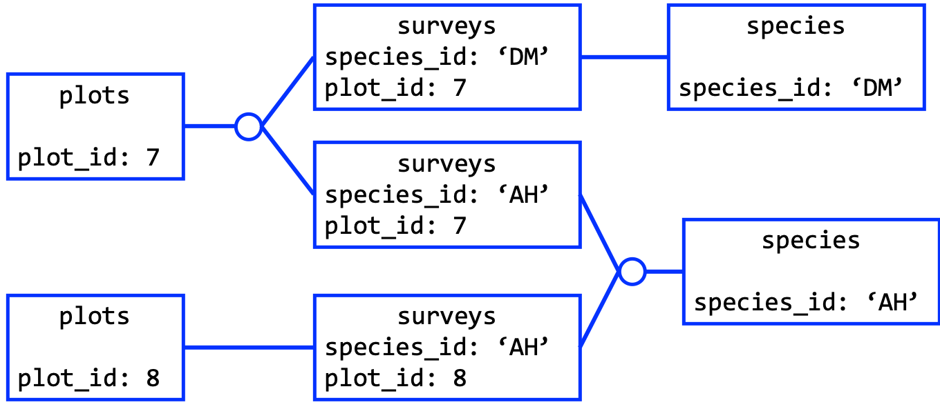
Surveys is an “association table” because it includes two foreign keys.
dbGetQuery(con, "SELECT weight, genus, plot_type
FROM surveys
JOIN plots
  ON surveys.plot_id = plots.plot_id
JOIN species
  ON surveys.species_id = species.species_id")
The resulting table could be the basis for the portal data.frame needed in the
R command lm(weight ~ genus + treatment, data = portal).
Summary
- concurrency
- reliability
- scaleability
Databases are a core element of a centralized workflow that requires simultaneous use by multiple members of a collaborative team. A server- based database such as Postgres will allow you to take advantage of concurrency features that prevent data corruption.
The ability to precisely define keys and data types is the primary database feature that guaranties reliability. As you develop scripts for analysis and vizualization, certainty that you’ll never encounter a “NaN” when you expect an Integer will prevent, or help you catch, bugs in your code.
The third major feature to motivate databae use, scaleability, remains for you to discover, using the tools from this lesson. Very large tables can be queried, sorted and combined quickly when the work is done by a powerful relational database management system (RDBMS), such as PostgreSQL.
If you need to catch-up before a section of code will work, just squish it's 🍅 to copy code above it into your clipboard. Then paste into your interpreter's console, run, and you'll be ready to start in on that section. Code copied by both 🍅 and 📋 will also appear below, where you can edit first, and then copy, paste, and run again.
# Nothing here yet!