Structure for Unstructured Data
Handouts for this lesson need to be saved on your computer. Download and unzip this material into the directory (a.k.a. folder) where you plan to work.
Structured Data
Structured data is a collection of multiple observations, each composed of one or more variables. Most analyses typically begin with structured data, the kind of tables you can view as a spreadhseet or numerical array.
The key to structure is that information is packaged into well-defined variables, e.g. the columns of a tidy data frame. Typically, it took someone a lot of effort to get information into a useful structure.
Well-defined Variables
Cox, M. 2015. Ecology & Society 20(1):63.
Variable Classification
Every variable fits within one of four categories—these are more general categories than you find when enumerating “data types” as understood by R or Python.
| Category | Definition |
|---|---|
| Numeric (or Interval) | Values separated by meaningful intervals/distances |
| Ordered | Ordered values without “distance” between them |
| Categorical | Finite set of distinct, un-ordered values |
| Qualitative | Unlimited, discrete, and un-ordered possibilities |
What we call quantitative data is actually any one of the first three.
- Qustion
- What is one example of each of the three types of quantitative data (interval, ordered, and categorical) a biological survey might produce?
- Answer
- For example, a fisheries survey might record size, age class (juvenile, adult), and species.
- Qustion
- What is an example of qualitative data the same biological survey might collect?
- Answer
- Surveys often collect descriptive data, e.g. description of micro-habitat where an organism was found.
Unstructured Data
Information that has not been carved up into variables is unstructured “data”— although some say that is a misnomer. Any field researcher knows when they are staring down raw information, and they are usually puzzling over how to collect or structure it.
Photo by trinisands / CC BY-SA and by Archives New Zealand / CC BY
Suppose you want to collect data on how businesses fail, so you download half a million e-mails from Enron executives that preceeded the energy company’s collapse in 2001.
Message-ID: <16986095.1075852351708.JavaMail.evans@thyme>
Date: Mon, 3 Sep 2001 12:24:09 -0700 (PDT)
From: greg.whalley@enron.com
To: kenneth.lay@enron.com, j..kean@enron.com
Subject: FW: Management Committee Offsite

I'm sorry I haven't been more involved is setting this up, but I think the
agenda looks kond of soft.  At a minimum, I would like to turn the schedule
around and hit the hard subjects like Q3, risk management, and ...
Structuring the data for analysis does not mean you quantify everything, although certainly some information can be quantified. Rather, turning unstructured information into structured data is a process of identifying concepts, definining variables, and assigning their values (i.e. taking measurements) from the text.
Possible examples for variables of different classes to associate with the Enron e-mails.
| Category | Example |
|---|---|
| Numeric (or Interval) | timestamp, e-mail length, occurrences of a given topic |
| Ordered | sender’s position in the company, step in process-tracing sequence of events |
| Categorical | sender’s department in the company, sender-recipient paris (e.g. network) |
| Qualitative | message subject matter, sender’s sentiment |
- Question
- What distinguishes data from unstructured information? What distinguishes qualitative data from unstructured information?
- Answer
- Data is the measurement of a variable that relates to a well-defined concept, while information is free of any analytical framework. Data is qualitative if its measurement could give any value and no measure of distance exists for any pair of values.
Processing of texts, surveys, recordings, etc. into variables (whether qualitative or not), is often described as qualitiative data analysis.
Computer Assisted QDA
- Coding
- Annotating a document collection by highlighting shared themes (CAQDA).
- e.g. highlighting sections of an email collection with “codes” or “themes”
- Scraping
- Process digitized information (websites, texts, images, recordings) into structured data.
- e.g. capture sender, date, and greeting from emails, storing values in a data frame
- Text Mining
- Processing text on the way to producing qualitative or quantitative data
- e.g. bag-of-words matrix
- Topic Modeling
- Algorithms for automatic coding of extensive document collections.
- e.g. latent Dirichlet allocation (LDA)
These are different ways of performing “feature engineering”, which requires both domain knowledge and programing skill. The feature engineer faces the dual challenges of linking concepts to variables and of creating structured data about these variables from a source of raw information.
Scraping
For text analysis, whether online or following document OCR, few tools are as useful for pulling out strings that represent a value than “regular expressions”.

by Randall Munroe / CC BY-NC
RegEx is a very flexible, and very fast, program for finding bits of text within a document that has particular features defined as a “pattern”.
| Pattern | String with match |
|---|---|
| Subject:.* | Subject: Re: TPS Reports |
| \$[0-9,]+ | The ransom of $1,000,000 to Dr. Evil. |
| \b\S+@\S+\b | E-mail info@sesync.org or tweet @SESYNC for details! |
Specifying these patterns correctly can be tricky. This is a useful site for testing out regex patterns specific to R.
Note that “\” must be escaped in R, so the third pattern does not look very nice in a R string.
library(stringr)

str_extract_all(
  'Email info@sesync.org or tweet @SESYNC for details!',
  '\\b\\S+@\\S+\\b')
[[1]]
[1] "info@sesync.org"
Continuing with the Enron emails theme, begin by collecting the documents for analysis with the tm package.
library(tm)

enron <- VCorpus(DirSource("data/enron"))
email <- enron[[1]]
> meta(email)
  author       : character(0)
  datetimestamp: 2020-07-02 17:09:24
  description  : character(0)
  heading      : character(0)
  id           : 10001529.1075861306591.txt
  language     : en
  origin       : character(0)
> content(email)
 [1] "Message-ID: <10001529.1075861306591.JavaMail.evans@thyme>"
 [2] "Date: Wed, 7 Nov 2001 13:58:24 -0800 (PST)"
 [3] "From: dutch.quigley@enron.com"
 [4] "To: frthis@aol.com"
 [5] "Subject: RE: seeing as mark won't answer my e-mails...."
 [6] "Mime-Version: 1.0"
 [7] "Content-Type: text/plain; charset=us-ascii"
 [8] "Content-Transfer-Encoding: 7bit"
 [9] "X-From: Quigley, Dutch </O=ENRON/OU=NA/CN=RECIPIENTS/CN=DQUIGLE>"
[10] "X-To: 'Frthis@aol.com@ENRON'"
[11] "X-cc: "
[12] "X-bcc: "
[13] "X-Folder: \\DQUIGLE (Non-Privileged)\\Quigley, Dutch\\Sent Items"
[14] "X-Origin: Quigley-D"
[15] "X-FileName: DQUIGLE (Non-Privileged).pst"
[16] ""
[17] "yes please on the directions"
[18] ""
[19] ""
[20] " -----Original Message-----"
[21] "From: \tFrthis@aol.com@ENRON  "
[22] "Sent:\tWednesday, November 07, 2001 3:57 PM"
[23] "To:\tsiva66@mail.ev1.net; MarkM@cajunusa.com; Wolphguy@aol.com; martier@cpchem.com; klyn@pdq.net"
[24] "Cc:\tRs1119@aol.com; Quigley, Dutch; john_riches@msn.com; jramirez@othon.com; bwdunlavy@yahoo.com"
[25] "Subject:\tRe: seeing as mark won't answer my e-mails...."
[26] ""
[27] "Kingwood Cove it is! "
[28] "Sunday "
[29] "Tee Time(s):  8:06 and 8:12 "
[30] "Cost - $33 (includes cart) - that will be be $66 for Mr. 2700 Huevos. "
[31] "ernie "
[32] "Anyone need directions?"
The RegEx pattern ^From: .* matches any whole line that begins with “From: “.
Parentheses cause parts of the match to be captured for substitution or
extraction.
match <- str_match(content(email), '^From: (.*)')
head(match)
     [,1]                            [,2]
[1,] NA                              NA
[2,] NA                              NA
[3,] "From: dutch.quigley@enron.com" "dutch.quigley@enron.com"
[4,] NA                              NA
[5,] NA                              NA
[6,] NA                              NA
Data Extraction
The meta object for each e-mail was sparsely populated, but some of those
variables can be extracted from the content.
enron <- tm_map(enron, function(email) {
  body <- content(email)
  match <- str_match(body, '^From: (.*)')
  match <- na.omit(match)
  meta(email, 'author') <- match[[1, 2]]
  return(email)
})
> email <- enron[[1]]
> meta(email)
  author       : dutch.quigley@enron.com
  datetimestamp: 2020-07-02 17:09:24
  description  : character(0)
  heading      : character(0)
  id           : 10001529.1075861306591.txt
  language     : en
  origin       : character(0)
Relational Data Extraction
Relational data are tables that establish a relationship between entities from other tables.
Suppose we have a table with a record for each unique email address in the Enron emails, then a second table with a record for each pair of addresses that exchanged a message is relational data.
> email <- enron[[2]]
> head(content(email))
[1] "Message-ID: <10016327.1075853078441.JavaMail.evans@thyme>"
[2] "Date: Mon, 20 Aug 2001 16:14:45 -0700 (PDT)"
[3] "From: lynn.blair@enron.com"
[4] "To: ronnie.brickman@enron.com, randy.howard@enron.com"
[5] "Subject: RE: Liquids in Region"
[6] "Cc: ld.stephens@enron.com, team.sublette@enron.com, w.miller@enron.com, "
This “To:” field is slightly harder to extract, because it may include multiple recipients.
get_to <- function(email) {
  body <- content(email)
  match <- str_detect(body, '^To:')
  if (any(match)) {
    to_start <- which(match)[[1]]
    match <- str_detect(body, '^Subject:')
    to_end <- which(match)[[1]] - 1
    to <- paste(body[to_start:to_end], collapse = '')
    to <- str_extract_all(to, '\\b\\S+@\\S+\\b')
    return(unlist(to))
  } else {
    return(NA)
  }
}
> get_to(email)
[1] "ronnie.brickman@enron.com" "randy.howard@enron.com"
Embed the above lines in a for loop to build an edge list for the network of e-mail senders and recipients.
edges <- lapply(enron, FUN = function(email) {
  from <- meta(email, 'author')
  to <- get_to(email)
  return(cbind(from, to))
})
edges <- do.call(rbind, edges)
edges <- na.omit(edges)
attr(edges, 'na.action') <- NULL
> dim(edges)
[1] 10493 2
The network package provides convenient tools for working with relational data.
library(network)

g <- network(edges)
plot(g)
- Question
- Is a network qualitative or quantitative data?
- Answer
- It certainly doesn’t fall into line with traditional statistical methods, but the variables involved are categorical. Methods for fitting models on networks (e.g. ERGMs) are an active research area.
Text Mining
Developing measurements of quantitative variables from unstructured information is another component of the “field-work” in research projects that rely on texts for empirical observations.
- Searching strings for patterns
- Cleaning strings of un-informative patterns
- Quantifying string occurrences and associations
- Interpretting the meaning of associated strings
Cleaning Text
Assuming the structured data in the Enron e-mail headers has been captured, strip down the content to the unstructured message.
enron <- tm_map(enron, function(email) {
  body <- content(email)
  match <- str_detect(body, '^X-FileName:')
  begin <- which(match)[[1]] + 1
  match <- str_detect(body, '^[>\\s]*[_\\-]{2}')
  match <- c(match, TRUE)
  end <- which(match)[[1]] - 1
  content(email) <- body[begin:end]
  return(email)
})
> email <- enron[[2]]
> content(email)
[1] ""
[2] "\tRonnie, I just got back from vacation and wanted to follow up on the discussion below."
[3] "\tHave you heard back from Jerry?  Do you need me to try calling Delaine again?  Thanks. Lynn"
[4] ""
Predefined Cleaning Functions
These are some of the functions listed by getTransformations.
library(magrittr)

enron_words <- enron %>%
  tm_map(removePunctuation) %>%
  tm_map(removeNumbers) %>%
  tm_map(stripWhitespace)
> email <- enron_words[[2]]
> content(email)
[1] ""
[2] " Ronnie I just got back from vacation and wanted to follow up on the discussion below"
[3] " Have you heard back from Jerry Do you need me to try calling Delaine again Thanks Lynn"
[4] ""
Customize document preparation with your own functions. The function must be
wrapped in content_transformer if designed to accept and return strings rather
than PlainTextDocuments.
remove_link <- function(body) {
  match <- str_detect(body, '(http|www|mailto)')
  body[!match]
}
enron_words <- enron_words %>%
  tm_map(content_transformer(remove_link))
Stopwords and Stems
Stopwords are the throwaway words that don’t inform content, and lists for different languages are complied within tm. Before removing them though, also “stem” the current words to remove plurals and other nuissances.
enron_words <- enron_words %>%
  tm_map(stemDocument) %>%
  tm_map(removeWords, stopwords("english"))
Document-Term Matrix
The “bag-of-words” model for turning a corpus into structured data is to simply count the word frequency in each document.
dtm <- DocumentTermMatrix(enron_words)
Long Form
The tidytext package converts the (wide) Document Term Matrix into a longer form table with a row for every document and term combination.
library(tidytext)
library(dplyr)

dtt <- tidy(dtm)
words <- dtt %>%
  group_by(term) %>%
  summarise(
    n = n(),
    total = sum(count)) %>%
  mutate(nchar = nchar(term))
The words data frame is more amenable to further inspection and
cleaning, such as removing outliers.
library(ggplot2)

ggplot(words, aes(x = nchar)) +
  geom_histogram(binwidth = 1)
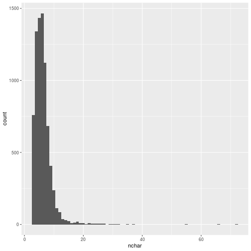
Words with too many characters are probably not actually words, and extremely uncommon words won’t help when searching for patterns.
dtt_trimmed <- words %>%
  filter(
    nchar < 16,
    n > 1,
    total > 3) %>%
  select(term) %>%
  inner_join(dtt)
Joining, by = "term"
Further steps in analyzing this “bag-of-words” require returning to the Document-Term-Matrix structure.
dtm_trimmed <- dtt_trimmed %>%
  cast_dtm(document, term, count)
> dtm_trimmed
<<DocumentTermMatrix (documents: 3756, terms: 2454)>>
Non-/sparse entries: 59821/9157403
Sparsity           : 99%
Maximal term length: 15
Weighting          : term frequency (tf)
Term Correlations
The findAssocs function checks columns of the document-term matrix for
correlations. For example, words that are associated with the name of the CEO,
Ken Lay.
word_assoc <- findAssocs(dtm_trimmed, 'ken', 0.6)
word_assoc <- data.frame(
  word = names(word_assoc[[1]]),
  assoc = word_assoc,
  row.names = NULL)
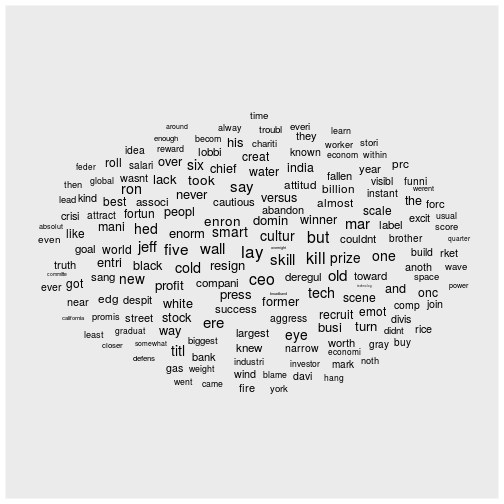
A “wordcloud” emphasizes those words that have a high co-occurence in the email corpus with the CEO’s first name.
library(ggwordcloud)

ggplot(word_assoc,
  aes(label = word, size = ken)) +
  geom_text_wordcloud_area()
Topic Modelling
Latent Dirichlet Allocation (LDA) is an algorithim that’s conceptually similar to dimensionallity reduction techniques for numerical data, such as PCA. Although, LDA requires you to determine the number of “topics” in a corpus beforehand, while PCA allows you to choose the number of principle components needed based on their loadings.
library(topicmodels)

seed = 12345
fit = LDA(dtm_trimmed, k = 5, control = list(seed=seed))
> terms(fit, 20)
      Topic 1    Topic 2 Topic 3      Topic 4    Topic 5
 [1,] "thank"    "get"   "market"     "price"    "mari"
 [2,] "lynn"     "will"  "monika"     "the"      "agreement"
 [3,] "will"     "know"  "enron"      "enron"    "enron"
 [4,] "pleas"    "can"   "financi"    "will"     "pleas"
 [5,] "meet"     "just"  "pulp"       "compani"  "thank"
 [6,] "can"      "like"  "includ"     "market"   "attach"
 [7,] "let"      "think" "compani"    "gas"      "will"
 [8,] "bill"     "dont"  "trader"     "trade"    "master"
 [9,] "know"     "time"  "skill"      "energi"   "know"
[10,] "need"     "look"  "load"       "deal"     "fax"
[11,] "fyi"      "want"  "trade"      "manag"    "let"
[12,] "ani"      "work"  "price"      "parti"    "ani"
[13,] "question" "call"  "inform"     "new"      "copi"
[14,] "call"     "one"   "north"      "transact" "need"
[15,] "schedul"  "good"  "oregon"     "this"     "corp"
[16,] "discuss"  "need"  "make"       "month"    "document"
[17,] "work"     "back"  "causholli"  "contract" "can"
[18,] "get"      "take"  "temperatur" "posit"    "send"
[19,] "group"    "day"   "data"       "use"      "sign"
[20,] "michell"  "hope"  "attach"     "servic"   "servic"
By assigning topic “weights” back to the documents, which gives an indication of how likely it is to find each topic in a document, you have engineered some numerical features associated with each document that might further help with classification or visualization.
email_topics <- as.data.frame(
  posterior(fit, dtm_trimmed)$topics)
> head(email_topics)
                                      1            2           3         4
15572442.1075858843984.txt 3.720195e-05 0.4526013220 0.229491023 0.3178332
3203154.1075852351910.txt  6.036603e-03 0.6220533207 0.120064073 0.2458096
13645178.1075839996540.txt 4.612527e-01 0.0029070018 0.051030738 0.3338006
22210912.1075858601602.txt 8.923614e-04 0.0008921769 0.012294932 0.9850281
2270209.1075858847824.txt  1.401818e-01 0.2407141202 0.002458558 0.6141870
26147562.1075839996615.txt 7.567838e-02 0.2396156416 0.101497075 0.5829608
                                      5
15572442.1075858843984.txt 3.721505e-05
3203154.1075852351910.txt  6.036383e-03
13645178.1075839996540.txt 1.510089e-01
22210912.1075858601602.txt 8.924571e-04
2270209.1075858847824.txt  2.458535e-03
26147562.1075839996615.txt 2.481385e-04
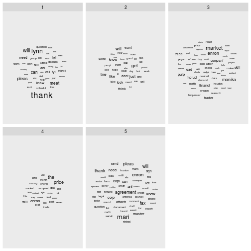
The challenge with LDA, as with any machine learning result, is interpretting the result. Are the “topics” recognizable by the words used?
library(ggwordcloud)

topics <- tidy(fit) %>%
  filter(beta > 0.004)

ggplot(topics,
  aes(size = beta, label = term)) +
  geom_text_wordcloud_area(rm_outside = TRUE) +
  facet_wrap(vars(topic))
Exercises
Exercise 1
Now that you’ve learned a bit about extracting strings, try using regex to extract money values from the e-mail body content.
Exercise 2
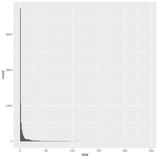
We plotted the number of characters in each word above. Word frequency in a document-term matrix might also be interesting. Try plotting a histogram of the number of times a word appears.
Exercise 3
What terms are associated with the word pipeline (“pipelin” after trimming)? How might you visualize this?
Solutions
Solution 1
str_extract_all(content(email), '\\$\\S+\\b')
[[1]]
character(0)

[[2]]
character(0)

[[3]]
character(0)

[[4]]
character(0)
Solution 2
ggplot(words, aes(x = total)) +
       geom_histogram(binwidth = 1)
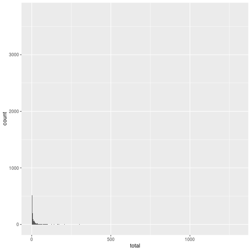
The frequency of some words isn’t very informative. You can filter by term or by total number of occurrences.
words_trim <- filter(words, total < 250)

ggplot(words_trim, aes(x = total)) +
       geom_histogram(binwidth = 1)
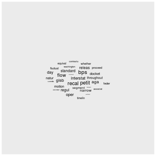
Solution 3
word_assoc <- findAssocs(dtm_trimmed, 'pipelin', 0.6)

word_assoc <- data.frame(word = names(word_assoc[[1]]),
                         assoc = word_assoc,
                         row.names = NULL)
ggplot(word_assoc, aes(label = word, size = pipelin)) +
       geom_text_wordcloud_area()
If you need to catch-up before a section of code will work, just squish it's 🍅 to copy code above it into your clipboard. Then paste into your interpreter's console, run, and you'll be ready to start in on that section. Code copied by both 🍅 and 📋 will also appear below, where you can edit first, and then copy, paste, and run again.
# Nothing here yet!