Introduction to Geospatial Data
Handouts for this lesson need to be saved on your computer. Download and unzip this material into the directory (a.k.a. folder) where you plan to work.
Lesson Objectives
- Meet the key R packages for geospatial analysis
- Learn basic wrangling of vector and raster data
- Distinguish “scriptable” tasks from desktop GIS tasks
Specific Achievements
- Create, load, and plot vector data types, or “features”
- Filter features based on associated data or on spatial location
- Perform geometric operations on polygons
- Load, manipulate, and extract raster data
R Packages
The key R packages for this lesson are
OSGeo Dependencies
Most R packages depend on other R packages. The sf and stars packages also depend on system libraries.
- GDAL for read/write in geospatial data formats
- GEOS for geometry operations
- PROJ for cartographic projections
System libraries cannot be installed by R’s install.packages(), but can be
bundled with these packages and for private use by them. Either way, the
necessary libraries are maintained by the good people at the Open Source
Geospatial Foundation for free and easy distribution. When
you load sf, it will return an error if any dependencies are not found.
Vector Data
The US Census website distributes county polygons (and much more) that are provided with the handouts. The sf package reads shapefiles (“.shp”) and most other vector data:
library(sf)

shp <- 'data/cb_2016_us_county_5m'
counties <- st_read(shp)
The object shp is a character string with the location of a folder that contains
the collection of individual files that make up a shapefile.
The counties object is a data.frame that includes a sfc, which stands for
“simple feature column”. This special column is usually called “geometry.”
> head(counties)
Simple feature collection with 6 features and 9 fields
Geometry type: MULTIPOLYGON
Dimension:     XY
Bounding box:  xmin: -114.7556 ymin: 29.26116 xmax: -81.10192 ymax: 38.77443
Geodetic CRS:  NAD83
  STATEFP COUNTYFP COUNTYNS       AFFGEOID GEOID      NAME LSAD       ALAND
1      04      015 00025445 0500000US04015 04015    Mohave   06 34475567011
2      12      035 00308547 0500000US12035 12035   Flagler   06  1257365642
3      20      129 00485135 0500000US20129 20129    Morton   06  1889993251
4      28      093 00695770 0500000US28093 28093  Marshall   06  1828989833
5      29      510 00767557 0500000US29510 29510 St. Louis   25   160458044
6      35      031 00929107 0500000US35031 35031  McKinley   06 14116799068
     AWATER                       geometry
1 387344307 MULTIPOLYGON (((-114.7556 3...
2 221047161 MULTIPOLYGON (((-81.52366 2...
3    507796 MULTIPOLYGON (((-102.042 37...
4   9195190 MULTIPOLYGON (((-89.72432 3...
5  10670040 MULTIPOLYGON (((-90.31821 3...
6  14078537 MULTIPOLYGON (((-109.0465 3...
In this case, we have a MULTIPOLYGON object which means that each row
has a column with information about the boundaries of a county polygon.
Geometry Types
Like any data.frame column, the geometry column is comprised of a single
data type. The “MULTIPOLYGON” is just one of several standard geometric data
types.
| Common Types | Description |
|---|---|
| POINT | zero-dimensional geometry containing a single point |
| LINESTRING | sequence of points connected by straight, non-self intersecting line pieces; one-dimensional geometry |
| POLYGON | sequence of points in closed, non-intersecting rings; the first denotes the exterior ring, any subsequent rings denote holes |
| MULTI* | set of * (POINT, LINESTRING, or POLYGON) |
The spatial data types are built upon each other in a logical way: lines are built from points, polygons are built from lines, and so on.
We can create any of these spatial objects from coordinates.
Here’s an sfc object with a single “POINT”, corresponding to SESYNC’s position
in degrees latitude and degrees longitude, with the same coordinate
reference system as the counties object.
sesync <- st_sfc(st_point(
    c(-76.503394, 38.976546)),
    crs = st_crs(counties))
Coordinate Reference Systems
A key feature of a geospatial data type is its associated CRS, stored in
Well Known Text (WKT) format. We can print the CRS of a spatial
object with st_crs().
> st_crs(counties)
Coordinate Reference System:
  User input: NAD83
  wkt:
GEOGCRS["NAD83",
    DATUM["North American Datum 1983",
        ELLIPSOID["GRS 1980",6378137,298.257222101,
            LENGTHUNIT["metre",1]]],
    PRIMEM["Greenwich",0,
        ANGLEUNIT["degree",0.0174532925199433]],
    CS[ellipsoidal,2],
        AXIS["latitude",north,
            ORDER[1],
            ANGLEUNIT["degree",0.0174532925199433]],
        AXIS["longitude",east,
            ORDER[2],
            ANGLEUNIT["degree",0.0174532925199433]],
    ID["EPSG",4269]]
The WKT contains parameters of the projection. The last line includes the EPSG ID, a numerical code indicating the coordinate reference system.
In order for two spatial objects to be comparable, they must be represented in the same coordinate reference system. This can be a geographic coordinate system or a projected coordinate system.
Geographic coordinate systems, like the one we saw when we called st_crs(counties), represent locations as degrees of latitude and longitude on the surface of the Earth, modeled as an ellipsoid (a slightly flattened sphere). The datum of a geographic coordinate system is the set of parameters representing the exact shape of the ellipsoid. The counties object uses the 1983 North American Datum, or NAD83 for short. Most world maps use the WGS84 datum.
A projected coordinate system converts geographical coordinates into Cartesian or rectangular (X, Y) coordinates for making two-dimensional maps. Since it is impossible to provide an exact two-dimensional representation of a three-dimensional object like Earth without losing some information, specialized projections were developed for different regions of the world and different analytical applications. For example, the Mercator projection (left) preserves shapes and angles, which is useful for navigation, but it greatly inflates areas at the poles. The Lambert equal-area projection (right) preserves areas at the cost of shape distortion away from its center.
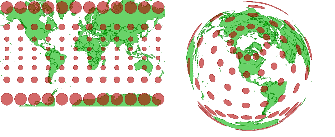
Projections can preserve shapes or areas, but not both.
Bounding Box
A bounding box for all features in an sf data frame is generated by st_bbox().
> st_bbox(counties)
      xmin       ymin       xmax       ymax
-179.14734  -14.55255  179.77847   71.35256
The bounding box is not a static attribute—it is determined on-the-fly for the entire table or any subset of features. In this example, we subset the United States counties by state ID 24 (Maryland).
Because the counties object is a kind of data.frame, we can use dplyr
verbs such as filter on it, just as we would with a non-spatial data frame. After
filtering, you can see that the bounding box is now much smaller.
library(dplyr)
counties_md <- filter(
  counties,
  STATEFP == '24')
> st_bbox(counties_md)
     xmin      ymin      xmax      ymax
-79.48765  37.91172 -75.04894  39.72312
Grid
A bounding box summarizes the limits, but is not itself a geometry (not a POINT or POLYGON), even though it has a CRS attribute.
> st_crs(st_bbox(counties_md))
Coordinate Reference System:
  User input: NAD83
  wkt:
GEOGCRS["NAD83",
    DATUM["North American Datum 1983",
        ELLIPSOID["GRS 1980",6378137,298.257222101,
            LENGTHUNIT["metre",1]]],
    PRIMEM["Greenwich",0,
        ANGLEUNIT["degree",0.0174532925199433]],
    CS[ellipsoidal,2],
        AXIS["latitude",north,
            ORDER[1],
            ANGLEUNIT["degree",0.0174532925199433]],
        AXIS["longitude",east,
            ORDER[2],
            ANGLEUNIT["degree",0.0174532925199433]],
    ID["EPSG",4269]]
We can use st_make_grid() to make a rectangular grid over a sf object.
The grid is a geometry—by default, a POLYGON.
grid_md <- st_make_grid(counties_md,
                        n = 4)
The st_make_grid() function draws a rectangular grid on the surface of a sphere. At the
relatively small spatial scale of the state of Maryland, the difference between a flat surface
and the surface of a sphere is minimal.
> grid_md
Geometry set for 16 features
Geometry type: POLYGON
Dimension:     XY
Bounding box:  xmin: -79.48765 ymin: 37.91172 xmax: -75.04894 ymax: 39.72312
Geodetic CRS:  NAD83
First 5 geometries:
POLYGON ((-79.48765 37.91172, -78.37797 37.9117...
POLYGON ((-78.37797 37.91172, -77.26829 37.9117...
POLYGON ((-77.26829 37.91172, -76.15862 37.9117...
POLYGON ((-76.15862 37.91172, -75.04894 37.9117...
POLYGON ((-79.48765 38.36457, -78.37797 38.3645...
Plot Layers
Spatial objects defined by sf are compatible with the plot
function. Setting the plot parameter add = TRUE allows an existing plot to
serve as a layer underneath the new one. The two layers should have the same
coordinate reference system.
The following code plots the grid first, then the ALAND (land area) column of counties_md.
This plots the county boundaries with the fill color of the polygons corresponding to the
area of the polygon.
The default color scheme means that larger counties appear yellow. Finally, we
overlay the point location of SESYNC.
plot(grid_md)
plot(counties_md['ALAND'],
     add = TRUE)
plot(sesync, col = "green",
     pch = 20, add = TRUE)
But note that the plot function won’t prevent you from layering up geometries
with different coordinate systems: you must safeguard your own plots from this
mistake. The arguments col and pch, by the way, are graphical parameters
used in base R, see ?par.
Customizing maps with ggplot2
The plot function is great for quick visualizations but the ggplot2
package gives you much more flexibility to customize your plots.
For those not familiar with ggplot2, a comprehensive introduction can be found in the Data Visualisation chapter of R for Data Science by Wickham and Grolemund, or check out SESYNC’s introductory ggplot2 lesson.
Producing any type of graph with ggplot2 requires a similar sequence of steps:
- Begin by calling
ggplot()and add any further plot elements by “adding” them with+; - Specify the dataset as well as aesthetic mappings (
aes), which associate variables in the data to graphical elements (xandyaxes, color, size and shape of points, etc.); - Add
geom_layers, which specify the type of graph; - Optionally, specify additional customization options such as axis names and limits, color themes, and more.
Let’s plot the Maryland county map with ggplot().
All sf objects can be plotted by adding geom_sf() layers to the plot,
which automatically associates the geometry column with the x and y coordinates of the features
in the correct projection. If there are multiple geom_sf() layers, ggplot() will
transform all layers to the projection system of the first layer added to the plot.
library(ggplot2)
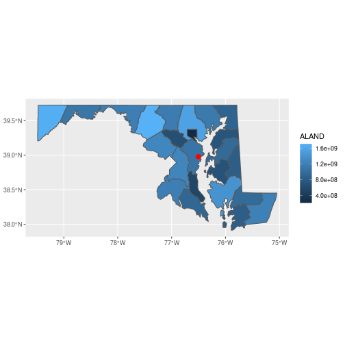
ggplot() +
geom_sf(data = counties_md,
aes(fill = ALAND)) +
geom_sf(data = sesync,
size = 3, color = 'red')
You can customize the plot theme and color scales, among other things.
theme_set(theme_bw())

ggplot() +
  geom_sf(data = counties_md,
          aes(fill = ALAND/1e6), color = NA) +
  geom_sf(data = sesync,
          size = 3, color = 'red') +
  scale_fill_viridis_c(name = 'Land area (sq. km)') +
  theme(legend.position = c(0.3, 0.3))
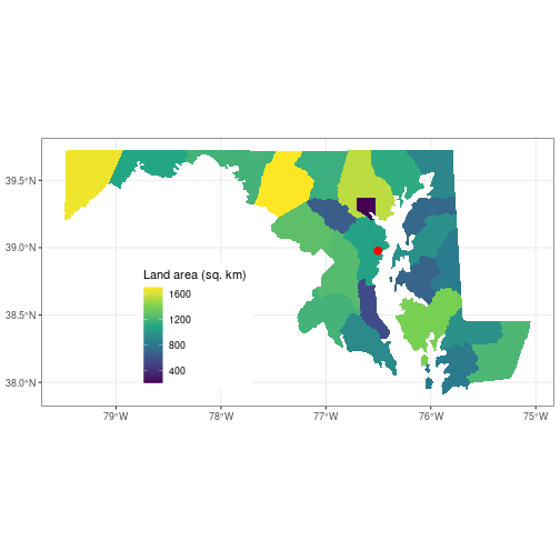
Here, we first set the plot theme for all other ggplot() plots we create in this
session to a black-and-white theme to get rid of the gray background.
Next, we divide the land area value by 1e6 to convert it to square km, then
specify color = NA for the county polygons so there is no border drawn around them.
We add a colorblind-friendly viridis fill scale for the polygons and add an
understandable legend title with the name argument to the fill scale. Finally
we move the legend to coordinates c(0.3, 0.3) in the panel (the legend position
can range from 0 to 1 on both axes). In all cases we add additional customization
elements to the base plot using +.
Spatial Subsetting
An object created with st_read() is a data.frame, which is why the dplyr
function filter used above on the non-geospatial column named STATEFP
worked normally. The function st_filter() does the equivalent of a filtering
operation on the geometry column, known as a spatial “overlay.”
> st_filter(counties_md, sesync)
Simple feature collection with 1 feature and 9 fields
Geometry type: MULTIPOLYGON
Dimension:     XY
Bounding box:  xmin: -76.84036 ymin: 38.71356 xmax: -76.39408 ymax: 39.2374
Geodetic CRS:  NAD83
  STATEFP COUNTYFP COUNTYNS       AFFGEOID GEOID         NAME LSAD      ALAND
1      24      003 01710958 0500000US24003 24003 Anne Arundel   06 1074553083
     AWATER                       geometry
1 447833714 MULTIPOLYGON (((-76.84036 3...
st_filter subsets the features of a sf object based on spatial (rather than numeric or
string) matching. Matching is implemented with functions like st_within(x, y). Here we
filtered the counties_md object to retain only the features that intersect with the
single point contained in the sesync object. Because sesync is a single point, this
results in a sfc with a single row.
The overlay functions in the sf package follow the pattern
st_predicate(x, y) and perform the test “x [is] predicate y”. Some key
examples are:
| st_intersects | boundary or interior of x intersects boundary or interior of y |
| st_within | interior and boundary of x do not intersect exterior of y |
| st_contains | y is within x |
| st_overlaps | interior of x intersects interior of y |
| st_equals | x has the same interior and boundary as y |
Coordinate Transforms
For the next part of this lesson, we import a new polygon layer corresponding to the 1:250k map of US hydrological units (HUC) downloaded from the United States Geological Survey.
shp <- 'data/huc250k'
huc <- st_read(shp)
Compare the coordinate reference systems of counties and huc by looking at
the WKT of both objects.
> st_crs(counties_md)
Coordinate Reference System:
  User input: NAD83
  wkt:
GEOGCRS["NAD83",
    DATUM["North American Datum 1983",
        ELLIPSOID["GRS 1980",6378137,298.257222101,
            LENGTHUNIT["metre",1]]],
    PRIMEM["Greenwich",0,
        ANGLEUNIT["degree",0.0174532925199433]],
    CS[ellipsoidal,2],
        AXIS["latitude",north,
            ORDER[1],
            ANGLEUNIT["degree",0.0174532925199433]],
        AXIS["longitude",east,
            ORDER[2],
            ANGLEUNIT["degree",0.0174532925199433]],
    ID["EPSG",4269]]
> st_crs(huc)
Coordinate Reference System:
  User input: NAD_1927_Albers
  wkt:
PROJCRS["NAD_1927_Albers",
    BASEGEOGCRS["NAD27",
        DATUM["North American Datum 1927",
            ELLIPSOID["Clarke 1866",6378206.4,294.9786982,
                LENGTHUNIT["metre",1]],
            ID["EPSG",6267]],
        PRIMEM["Greenwich",0,
            ANGLEUNIT["Degree",0.0174532925199433]]],
    CONVERSION["unnamed",
        METHOD["Albers Equal Area",
            ID["EPSG",9822]],
        PARAMETER["Latitude of false origin",23,
            ANGLEUNIT["Degree",0.0174532925199433],
            ID["EPSG",8821]],
        PARAMETER["Longitude of false origin",-96,
            ANGLEUNIT["Degree",0.0174532925199433],
            ID["EPSG",8822]],
        PARAMETER["Latitude of 1st standard parallel",29.5,
            ANGLEUNIT["Degree",0.0174532925199433],
            ID["EPSG",8823]],
        PARAMETER["Latitude of 2nd standard parallel",45.5,
            ANGLEUNIT["Degree",0.0174532925199433],
            ID["EPSG",8824]],
        PARAMETER["Easting at false origin",0,
            LENGTHUNIT["metre",1],
            ID["EPSG",8826]],
        PARAMETER["Northing at false origin",0,
            LENGTHUNIT["metre",1],
            ID["EPSG",8827]]],
    CS[Cartesian,2],
        AXIS["(E)",east,
            ORDER[1],
            LENGTHUNIT["metre",1,
                ID["EPSG",9001]]],
        AXIS["(N)",north,
            ORDER[2],
            LENGTHUNIT["metre",1,
                ID["EPSG",9001]]]]
The Census data uses unprojected (longitude, latitude) coordinates, but huc is
in an Albers equal-area projection (indicated as PROJECTION["Albers_Conic_Equal_Area"]).
Maps of the continental United States often use the Albers projection.
Important Note: Until recently, coordinate systems were represented with PROJ.4 strings, but in 2020 the developers of sf replaced them with the more precise Well Known Text format. We will still use PROJ.4 strings in this lesson to transform coordinate systems. Keep in mind, though, that development of geospatial R packages is always ongoing, and this lesson may be updated in the future to reflect that development.
The function st_transform() converts an sfc between coordinate reference
systems, specified with the parameter crs = x. A numeric x must be a valid
EPSG code; a character x is interpreted as a PROJ.4 string.
For example, the unprojected CRS of counties can be represented as the
PROJ.4 string "+proj=longlat +datum=NAD83 +no_defs". This character string
is a list of parameters that correspond to the EPSG code 4269.
You can transform objects to that projection using the PROJ.4 string as the argument
to crs, or by typing crs = 4269. The EPSG code or PROJ.4 string is translated
to the WKT format.
Not all projections have an EPSG code.
The projection in the PROJ.4 string below does not have an
EPSG code, for example. We’ll transform all the sfc objects to this
projection because it is the one used by the NLCD raster layer we’ll
introduce later in this lesson.
prj <- '+proj=aea +lat_1=29.5 +lat_2=45.5 \
        +lat_0=23 +lon_0=-96 +x_0=0 +y_0=0 \
        +datum=WGS84 +units=m +no_defs'
PROJ.4 strings contain a reference to the type of projection—this one is another
Albers equal-area, as indicated by +proj=aea—along with numeric parameters associated with that
projection. An additional important parameter that may differ between two
coordinate systems is the “datum”, which indicates the standard by which the
irregular surface of the Earth is approximated by an ellipsoid in the
coordinates themselves.
Use st_transform() to assign the two layers and SESYNC’s location
to a common projection string (prj).
This takes a few moments, as it recalculates coordinates for
every vertex in the sfc.
counties_md <- st_transform(
  counties_md,
  crs = prj)
huc <- st_transform(
  huc,
  crs = prj)
sesync <- st_transform(
  sesync,
  crs = prj)
Now that the three objects share a projection, we can plot the county boundaries, watershed boundaries, and SESYNC’s location on a single map.
plot(st_geometry(counties_md))
plot(st_geometry(huc),
     border = 'blue', add = TRUE)
plot(sesync, col = 'green',
     pch = 20, add = TRUE)
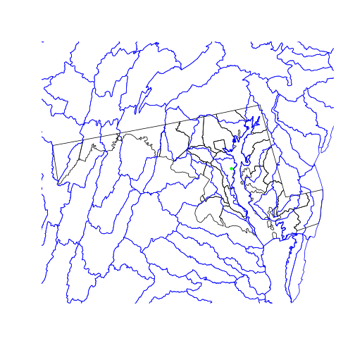
We use the st_geometry() function on the two polygon layers we plot, which
only plots the polygon boundaries (the geometry column) rather than filling
the areas with colors. st_geometry(x) is equivalent to x$geometry.
Geometric Operations
The data for a map of watershed boundaries within the state of MD is all here:
in the country-wide huc and in the state boundary “surrounding” all of
counties_md. To get just the HUCs inside Maryland’s borders:
- remove the internal county boundaries within the state
- clip the hydrological areas to their intersection with the state
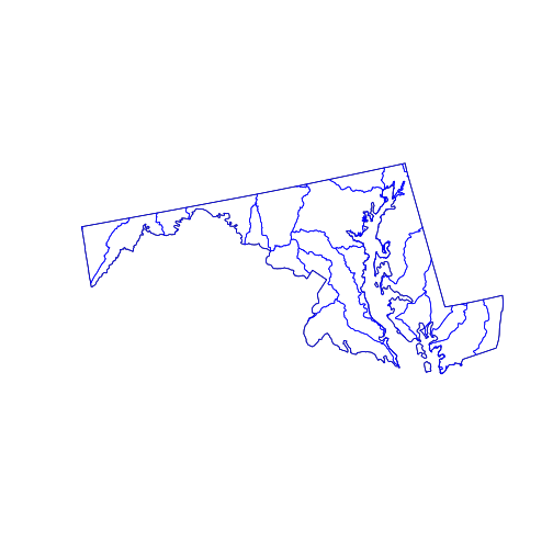
The first step is a spatial union operation: we want the resulting object to
combine the area covered by all the multipolygons in counties_md.
state_md <- st_union(counties_md)
plot(state_md)

To perform a union of all sub-geometries in a single sfc, we use the
st_union() function with a single argument. The output, state_md, is a new
sfc that is no longer a column of a data frame. Tabular data can’t safely
survive a spatial union because the polygons corresponding to the attributes
in the table have been combined into a single larger polygon. So the data frame
columns are discarded.
The second step is a spatial intersection, since we want to limit the
polygons to areas covered by both huc and state_md.
huc_md <- st_intersection(
  huc,
  state_md)
Warning: attribute variables are assumed to be spatially constant throughout all
geometries
plot(state_md)
plot(st_geometry(huc_md), border = 'blue',
     col = NA, add = TRUE)
The st_intersection() function intersects its first argument with the second.
The individual hydrological units are preserved but any part of them (or any
whole polygon) lying outside the state_md polygon is cut from the output. The
attribute data remains in the corresponding records of the data.frame, but (as
warned) has not been updated. For example, the “AREA” attribute of any clipped
HUC does not reflect the area of the new, smaller polygon.
The sf package provides many functions dealing with distances and areas.
st_buffer: to create a buffer of specific width around a geometryst_distance: to calculate the shortest distance between geometriesst_area: to calculate the area of polygons
These functions were recently updated to use geodesic distances that account for Earth’s curvature, making them accurate even at large spatial scales. You might also want to check out the geosphere package.
Raster Data
Raster data is a matrix or cube with additional spatial metadata (e.g. extent,
resolution, and projection) that allows its values to be mapped onto geographical
space. The stars package provides the read_stars() function
for reading the many formats of such data.
In the past (from 2010 to 2020), the raster package was the primary R package for reading and working with raster data. Recently, the developers of sf released stars (Spatio-Temporal ARrayS). It is integrated more closely with sf and related packages, as well as with the “tidyverse” family of packages, and has significant performance advantages. Another new alternative is terra, created by the developer of raster. Older versions of this lesson use raster, and you may come across the raster package when searching for help on geospatial data analysis in R. Nevertheless we recommend terra or stars because of their simplicity and speed advantages, and also because they are more likely to be updated and maintained in the future.
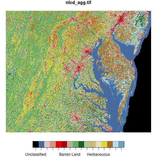
The National Land Cover Database is a 30m resolution grid of cells classified as forest, crops, wetland, developed, etc., across the continental United States. The file provided in this lesson is cropped and reduced to a lower resolution in order to speed processing.
library(stars)
nlcd <- read_stars("data/nlcd_agg.tif", proxy = FALSE)
nlcd <- droplevels(nlcd)
Here we set proxy = FALSE because this is a small example raster that we can
load into working memory.
If proxy = TRUE, raster data is not loaded into working memory, as you can confirm
by checking the R object size with object.size(nlcd). This means that unlike
most analyses in R, you can actually process raster datasets larger than the RAM
available on your computer; stars automatically loads pieces of the
data and computes on each of them in sequence. By default, stars will load small
rasters into working memory and large rasters as proxies unless you specify otherwise.
Also note that the nlcd_agg.tif file is accompanied by a metadata file called
nlcd_agg.tif.aux.xml that stores information including descriptive names for the different
land cover classes.
We need to call droplevels(nlcd) to remove empty factor levels. The
NLCD 2016 legend
classification codes are not sequential and begin with 11, but factor levels in R begin with 1.
Using droplevels gets rid of the empty levels so that the legends on the plots
we will make in a moment do not include blank levels.
The default print method for a stars raster object is a summary of metadata contained
in the raster file.
> nlcd
stars object with 2 dimensions and 1 attribute
attribute(s), summary of first 1e+05 cells:
                  nlcd_agg.tif
 Deciduous Forest        :32576
 Cultivated Crops        :13014
 Developed, Open Space   :11063
 Hay/Pasture             :10729
 Mixed Forest            : 9260
 Developed, Low Intensity: 8034
 (Other)                 :15324
dimension(s):
  from   to  offset delta                    refsys point values x/y
x    1 3004 1394535   150 Albers_Conical_Equal_Area FALSE   NULL [x]
y    1 2514 2101515  -150 Albers_Conical_Equal_Area FALSE   NULL [y]
The plot method interprets the pixel values of the raster matrix according to a
pre-defined color scheme.
> plot(nlcd)
downsample set to c(5,5)
The st_crop() function trims a stars raster object to the dimensions of a given
spatial object or bounding box.
Here we crop the NLCD raster
to the bounding box of the huc_md polygon, then display both layers on the same map.
(We can plot polygon and raster layers together on the same map, just like we can plot
multiple polygon layers—as long as they have the same coordinate reference system!)
Because ggplot2 does not automagically recognize the predefined color scheme from the
original image file, we have to extract the color scheme using
attr(nlcd[[1]], 'colors') and use it as an argument to scale_fill_manual().
md_bbox <- st_bbox(huc_md)
nlcd <- st_crop(nlcd, md_bbox)

ggplot() +
  geom_stars(data = nlcd) +
  geom_sf(data = huc_md, fill = NA) +
  scale_fill_manual(values = attr(nlcd[[1]], 'colors'))

A raster is fundamentally a data matrix, and individual pixel values can be
extracted by regular matrix subscripting. The matrix of pixel values is found
in list element [[1]] of a stars object. For example, the value of
the bottom-left corner pixel:
> nlcd[[1]][1, 1]
[1] Herbaceuous
16 Levels: Unclassified Open Water ... Emergent Herbaceuous Wetlands
The index [1, 1] corresponds to the bottom left pixel because the raster
represents a two-dimensional image with x and y coordinates. The origin
of the axes is at the bottom left.
For this particular dataset, land cover class is represented as a factor
variable. We can display the factor levels of nlcd[[1]]:
> levels(nlcd[[1]])
 [1] "Unclassified"                  "Open Water"
 [3] "Developed, Open Space"         "Developed, Low Intensity"
 [5] "Developed, Medium Intensity"   "Developed, High Intensity"
 [7] "Barren Land"                   "Deciduous Forest"
 [9] "Evergreen Forest"              "Mixed Forest"
[11] "Shrub/Scrub"                   "Herbaceuous"
[13] "Hay/Pasture"                   "Cultivated Crops"
[15] "Woody Wetlands"                "Emergent Herbaceuous Wetlands"
Writing pull(nlcd) is equivalent to nlcd[[1]]. This can be useful if
you are extracting values from a raster as part of a “pipe.” For example,
nlcd %>% pull %>% levels would give the same result as the code above.
Raster Math
Mathematical functions called on a raster get applied to each pixel. For a
single raster r, the function log(r) returns a new raster where each pixel’s
value is the log of the corresponding pixel in r.
Likewise, addition with r1 + r2 creates a raster where each pixel is the sum of the
values from r1 and r2, and so on. Naturally, spatial attributes of rasters
(e.g. extent, resolution, and projection) must match for functions that operate
pixel-wise on multiple rasters.
Logical operations work too: r1 > 5 returns a raster with pixel values TRUE
or FALSE and is often used to “mask” a raster, or remove pixels that don’t
meet a certain logical condition.
forest_types <- c('Evergreen Forest', 'Deciduous Forest', 'Mixed Forest')
forest_mask <- nlcd
forest_mask[!(forest_mask %in% forest_types)] <- NA
plot(forest_mask)
downsample set to c(3,3)
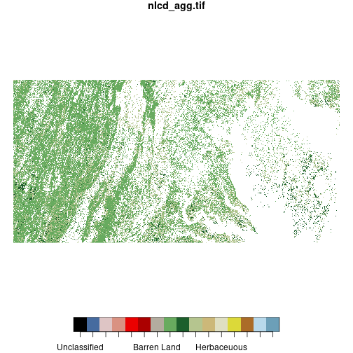
We define a vector including the levels of nlcd representing three types of forest and
create a copy of nlcd called forest_mask. We “mask out” all pixels in forest_mask that do not meet
the logical condition forest %in% forest_types, setting them to NA. (The ! negates a
logical condition.) This results in a raster
where all pixels that are not classified as forest are removed.
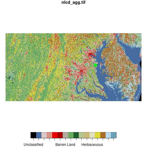
To further reduce the resolution of the nlcd raster, the st_warp()
function combines values in a block of a given size using a given method.
nlcd_agg <- st_warp(nlcd,
                    cellsize = 1500,
                    method = 'mode',
                    use_gdal = TRUE)

nlcd_agg <- droplevels(nlcd_agg)
levels(nlcd_agg[[1]]) <- levels(nlcd[[1]])

plot(nlcd_agg)
Here, cellsize = 1500 specifies that the raster should be downsampled to 1500-meter
pixel size. The input raster has 150-meter resolution, so this will convert
10-by-10 blocks of pixels to single pixels.
The argument method = 'mode' indicates that the aggregated value is the
mode of the input pixels making up each output pixel
(averaging would not work since land cover is a categorical variable).
use_gdal = TRUE specifies to use the GDAL system library “behind the scenes” to
do the aggregation, which is needed for aggregation methods including mode.
Unfortunately, the call to GDAL strips away the land cover class names so we
replace them by dropping unused levels with droplevels() and then replacing the names
with levels().
Crossing Rasters with Vectors
Raster and vector geospatial data in R require different packages. The creation of geospatial tools in R has been a community effort, and not necessarily a well-organized one. Development is still ongoing on many packages dealing with raster and vector data. The stars package has not yet released a “version 1.0” (it’s at 0.5 as of this writing). Developers are working hard on improving the package but if you notice any issues or bugs, report them on their GitHub repo.
Although not needed in this lesson, you may notice when using some older geospatial packages that it is necessary to
convert a vector object from sf (class beginning with sfc*) to sp
(class beginning with Spatial*). sp is an older package that was replaced
by sf, and many geospatial packages still work with sp objects.
You can do this by calling sp_object <- as(sf_object, 'Spatial'). You may also
need to convert a stars object to a Raster* class object, which you can do
by calling stars_object <- as(sf_object, 'Raster').
The st_extract() function allows subsetting and aggregation of raster values based
on a vector spatial object. For example we might want to extract the NLCD land cover
class at SESYNC’s location.
plot(nlcd, reset = FALSE)
downsample set to c(3,3)
plot(sesync, col = 'green',
     pch = 16, cex = 2, add = TRUE)
When we use plot() to combine raster and vector layers we need to set reset = FALSE on
the first layer we plot so that additional objects can be added to the plot.
Call st_extract() on the nlcd raster and the sfc object containing SESYNC’s point location.
When extracting by point locations, the result is another sfc with POINT geometry and
a column containing the pixel values from the raster at each point.
sesync_lc <- st_extract(nlcd, sesync)
> sesync_lc
Simple feature collection with 1 feature and 1 field
Geometry type: POINT
Dimension:     XY
Bounding box:  xmin: 1661671 ymin: 1943333 xmax: 1661671 ymax: 1943333
CRS:           +proj=aea +lat_1=29.5 +lat_2=45.5
        +lat_0=23 +lon_0=-96 +x_0=0 +y_0=0
        +datum=WGS84 +units=m +no_defs
                 nlcd_agg.tif                geometry
1 Developed, Medium Intensity POINT (1661671 1943333)
Instead of returning a point geometry, you might want to mask a raster by a point geometry instead.
You can use the indexing operator [] to do this. This will set
all pixels in the raster not overlapping the point geometry to NA.
> nlcd[sesync]
stars object with 2 dimensions and 1 attribute
attribute(s):
                     nlcd_agg.tif
 Developed, Medium Intensity:1
 Unclassified               :0
 Open Water                 :0
 Developed, Open Space      :0
 Developed, Low Intensity   :0
 Developed, High Intensity  :0
 (Other)                    :0
dimension(s):
  from   to  offset delta                    refsys point values x/y
x 1781 1781 1394535   150 Albers_Conical_Equal_Area FALSE   NULL [x]
y 1055 1055 2101515  -150 Albers_Conical_Equal_Area FALSE   NULL [y]
To extract with a polygon, first subset the raster by the polygon geometry. For example
here we subset the NLCD raster by the first row of counties_md
(Baltimore City), resulting in a raster with smaller dimensions that we can plot.
baltimore <- nlcd[counties_md[1, ]]
plot(baltimore)
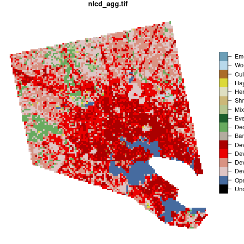
The expression nlcd[counties_md[1, ]] is equivalent to st_crop(nlcd, counties_md[1, ]).
The version with st_crop() is a bit easier to use with pipes.
Here we use a pipe to crop the NLCD raster to the boundaries of Baltimore City, pull the values as a matrix, and tabulate them.
nlcd %>%
  st_crop(counties_md[1, ]) %>%
  pull %>%
  table
.
                 Unclassified                    Open Water
                            0                           580
        Developed, Open Space      Developed, Low Intensity
                         1784                          2276
  Developed, Medium Intensity     Developed, High Intensity
                         2414                          2067
                  Barren Land              Deciduous Forest
                           62                           563
             Evergreen Forest                  Mixed Forest
                            8                            78
                  Shrub/Scrub                   Herbaceuous
                            3                             8
                  Hay/Pasture              Cultivated Crops
                           26                            22
               Woody Wetlands Emergent Herbaceuous Wetlands
                           26                             2
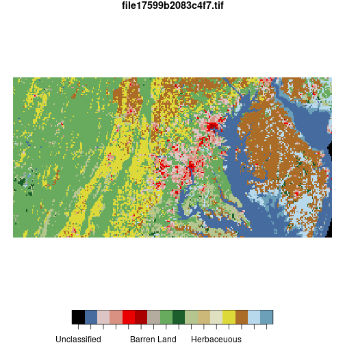
To get a summary of raster values for each polygon in an sfc
object, use aggregate() and specify an aggregation function FUN. This
example gives the most common land cover type for each polygon in huc_md.
mymode <- function(x) names(which.max(table(x)))

modal_lc <- aggregate(nlcd_agg, huc_md, FUN = mymode)
The stars package (and base R for that matter) currently have no built-in mode function
so we define a simple one here and pass it to aggregate().
The result is a stars object. We can convert it to an sfc object containing polygon
geometry.
> st_as_sf(modal_lc)
Simple feature collection with 30 features and 1 field
Geometry type: GEOMETRY
Dimension:     XY
Bounding box:  xmin: 1396621 ymin: 1837626 xmax: 1797030 ymax: 2037741
CRS:           +proj=aea +lat_1=29.5 +lat_2=45.5
        +lat_0=23 +lon_0=-96 +x_0=0 +y_0=0
        +datum=WGS84 +units=m +no_defs
First 10 features:
   file17599b2083c4f7.tif                       geometry
1        Deciduous Forest MULTIPOLYGON (((1683575 203...
2             Hay/Pasture MULTIPOLYGON (((1707075 202...
3        Deciduous Forest POLYGON ((1563404 2008455, ...
4        Cultivated Crops POLYGON ((1701439 2037188, ...
5        Deciduous Forest POLYGON ((1441528 1985664, ...
6             Hay/Pasture POLYGON ((1610557 2016043, ...
7        Deciduous Forest POLYGON ((1610557 2016043, ...
8              Open Water MULTIPOLYGON (((1691021 201...
9        Deciduous Forest POLYGON ((1496410 1995810, ...
10       Deciduous Forest POLYGON ((1468299 1990565, ...
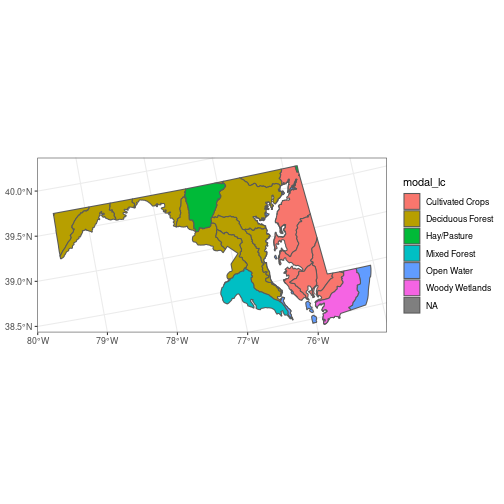
Alternatively, we can extract the values from the stars object, add them as a new
column to huc_md, and plot:
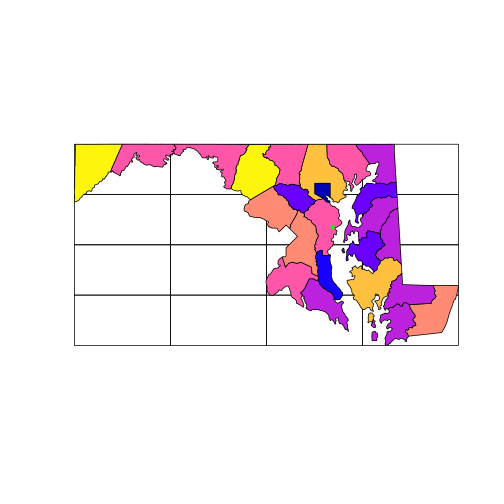
huc_md <- huc_md %>%
  mutate(modal_lc = modal_lc[[1]])

ggplot(huc_md, aes(fill = modal_lc)) +
  geom_sf()
Interactive Maps
The mapview package is a great way to quickly view vector or raster data interactively, using a JavaScript library called leaflet. It produces interactive maps (with controls to zoom, pan and toggle layers) combining local data with base layers from web mapping services.
You can pass a vector or raster object to the mapview() function, which will create a map
centered over your spatial object over a base tiled map.
By default, it imports tiles from Carto but you can switch to OpenStreetMap, ESRI World Imagery, or OpenTopoMap by clicking on the tile icon in the upper left.
library(mapview)
Warning: multiple methods tables found for 'crop'
Warning: multiple methods tables found for 'extend'
mapview(huc_md)
We are using all default arguments for mapview(), but there are
many additional options that you can set. You can see a few of them in the
next example.
The map shows up in the “Viewer” tab in RStudio because, like everything with
JavaScript, it relies on your browser to render the image.
Additional spatial datasets (points, lines, polygons, rasters) in your R environment can
be added as map layers using +. Mapview will try to make the necessary
transformation to display your data in EPSG:3857.
mapview(nlcd_agg, legend = FALSE, alpha = 0.5,
        map.types = 'OpenStreetMap') +
    mapview(huc_md, legend = FALSE, alpha.regions = 0.2)
The EPSG:3857 projection, also known as Web Mercator, will look familiar to you if you’ve ever used Google Maps, Apple Maps, or OpenStreetMap. It’s used in practically all online map applications. It sacrifices a little accuracy to dramatically speed up page load times.
If you hover your mouse over one of the polygon features, you can see the polygon ID, and if you click on it, a pop-up appears with more details. You can zoom and pan the map with your mouse; restore the zoom to the default or zoom in on one map layer using one of the buttons at the bottom of the pane.
Notice also that we passed a few extra arguments to mapview() to customize the map.
Setting legend = FALSE gets rid of the large legend panel. Setting
alpha for a raster layer and alpha.regions for a polygon layer to low values
makes them more transparent so that we can see the underlying map.
Finally, setting map.types changes which base map displays by default.
See ?mapview and ?mapviewOptions for more options.
The mapview package uses the R package leaflet behind the scenes, which is an R interface to the leaflet JavaScript library. mapview is great for quick dives into your data, but leaflet provides a lot more options and customizability if you want to embed maps into websites. For an in-depth leaflet tutorial, check out the SESYNC lesson on leaflet in R.
Resources
- stars package vignette.
- R.S. Bivand, E.J. Pebesma and V. Gómez-Rubio (2013) Applied Spatial Data Analysis with R. UseR! Series, Springer.
- R. Lovelace et al., Geocomputation with R
- Center for Spatial Data Science. Tutorials - Learn Spatial Analysis
- Spatial Data Science with R and terra uses the terra package instead of stars
- CRAN Task View: Analysis of Spatial Data
- P. Marchand. Introduction to geospatial data analysis in R
- “Legacy” version of this lesson uses the raster package instead of stars
More packages to try out
- exactextractr: quickly summarizes rasters across polygons
- rasterVis: supplements raster and terra for improved visualizations
Exercises
Exercise 1
Produce a map of Maryland counties with the county that contains SESYNC colored in red, using either plot() or ggplot(). Hint: use st_filter() to find the county that contains SESYNC.
Exercise 2
Use st_buffer() to create a 5km buffer around the state_md border and plot it as a dotted line over the true state border. Use either plot(..., lty = 'dotted') or ggplot() with geom_sf(..., linetype = 'dotted'). Hint: check the layer’s units with st_crs() and express any distance in those units.
Exercise 3
The function map from the purrr package aggregates across an entire raster. Use it to figure out the proportion of nlcd pixels that are covered by deciduous forest (value = 'Deciduous Forest'). Hint: use == to make a raster where only deciduous forest cells are TRUE, then use map to apply the function mean to that raster.
Solutions
Solution 1
> counties_sesync <- st_filter(counties_md, sesync)
Solution with plot():
> plot(st_geometry(counties_md))
> plot(counties_sesync, col = 'red', add = TRUE)
> plot(sesync, col = 'green', pch = 20, add = TRUE)
Solution with ggplot():
> ggplot() +
+   geom_sf(data = counties_md, fill = NA) +
+   geom_sf(data = counties_sesync, fill = 'red') +
+   geom_sf(data = sesync, color = 'green')
Solution 2
> bubble_md <- st_buffer(state_md, 5000)
Solution with plot()
> plot(state_md)
> plot(bubble_md, lty = 'dotted', add = TRUE)
Solution with ggplot()
> ggplot() +
+   geom_sf(data = st_geometry(state_md)) +
+   geom_sf(data = bubble_md, linetype = 'dotted', fill = NA)
Solution 3
> library(purrr)
> map(nlcd == 'Deciduous Forest', mean)
If you need to catch-up before a section of code will work, just squish it's 🍅 to copy code above it into your clipboard. Then paste into your interpreter's console, run, and you'll be ready to start in on that section. Code copied by both 🍅 and 📋 will also appear below, where you can edit first, and then copy, paste, and run again.
# Nothing here yet!